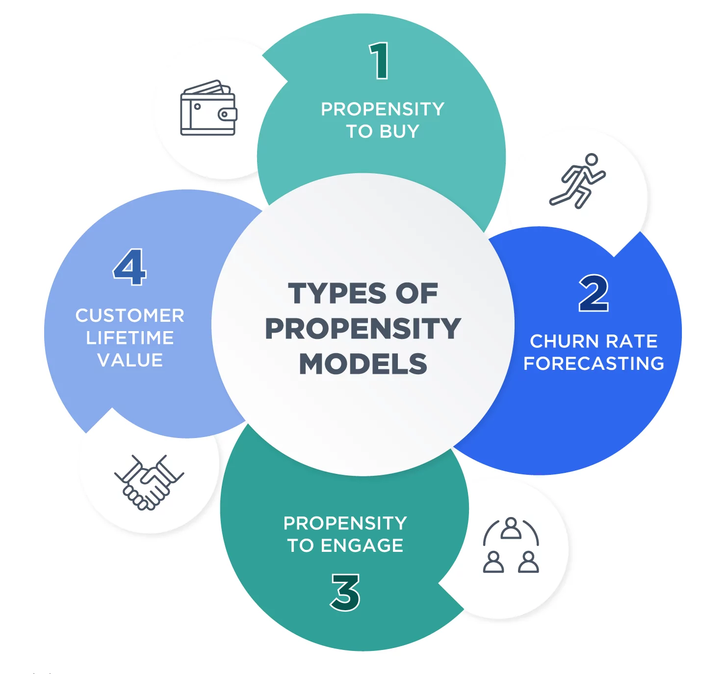
Why Propensity-to-Buy Prospecting Matters

• Precision Resource Allocation: It identifies the prospects with the highest likelihood to purchase, allowing marketing and sales teams to focus their budget and energy where it will yield the highest return.
• Relevant Communication: By profiling high-potential prospects with high P2B scores marketers can craft relevant communications to overcome the anonymity associated with a “cold start”.
• Optimized Marketing Frequency: It prevents “over-indexing” or inundating low-potential prospects with excessive outreach, identifying the “tipping point” where increased contact frequency decreases the probability of a sale.
• Foundation for Advanced Metrics: Propensity-to-Buy (P2B) generates the critical probability scores required to calculate more complex financial models, such as Customer Lifetime Value (CLV), effectively bridging the gap between marketing activity and long-term profitability.
• Strategic Profiling: It isolates high-propensity populations to uncover the influential variables (e.g., job title, industry, demographics, or financial stability) that define the “ideal” customer profile for future targeting.

---

A propensity-to-buy (P2B) model scores the likelihood that a lead, prospect, or customer will convert, respond, or churn. It is typically a statistical or machine-learning binary classifier that uses everything you know about a lead, prospect, or customer to make that prediction. Every propensity model I have built in twenty+ years of doing this has started with the assumption that the people or businesses we are scoring have a past. However, when we look at the data, we often find that the most influential information needed to predict purchase or response lies with customers and is largely absent from prospects.

Recency, frequency, monetary value. I wrote about the power of RFM Segmentation. Then we have marketing responsiveness (prior campaign response). Product ownership. Customer support tickets. The entire apparatus of behavioral scoring rests on the premise that this person, buying group, company or account has done something before, and that what they did predicts what they will do next.

Then marketing asks you to score the prospect file for a new customer acquisition program, and the assumption collapses and uncertainty increases.

This article asks a specific question: should never-contacted prospects be scored with their own model, separate from customers with contact, marketing and purchasing history? Instead of running one model across the entire database and hoping the statistics sort it out, we can separate people with history from those without it and measure exactly what that history is worth.

The answer can make a significant difference in GTM effectiveness, and the reason offers a lesson in metric selection that applies well beyond this dataset. In my experience, past purchase recency, frequency, and monetary value (RFM) are such powerful predictors that high-potential prospects critical for new customer acquisition will remain buried in the lower deciles of a blended prospect + customer scored list. They will be overlooked, and new customer acquisition will take a backseat to existing-customer installed-base cross-sell/up-sell marketing.

---

A Note on Data Integrity and Ethics

To maintain the highest ethical standards and ensure zero overlap with proprietary information from past or current employers, the analysis in this series is conducted on a publicly available open-source dataset from the University of California at Irvine’s Machine Learning Archive.

In this article I use the UCI Bank Marketing dataset — 45,211 records from a Portuguese retail bank’s term-deposit telemarketing campaigns, published by Moro, Rita, and Cortez (2014). Readers of my past articles will know that I have found this dataset excellent for a wide range of marketing data science use. Generally speaking, I always use public or synthetic data and have used many of the UCI datasets because they are (a) extremely popular for use by academic institutions and (b) a good fit for a wide range of modeling.

---

The Dataset and Target Variable

The target is binary: did the customer subscribe to a term deposit (y = yes) or not. Across the full file the base rate is 11.7%. The dataset was trained on the full file.  However, 81% of that file had never been contacted before. So, for most of the population the three key features: promotion days, previous contact and outcome were all null or zero.  So we have zero variance and zero information from the most powerful features for predicting purchase in my experience. Here is a sample of the data to illustrate:

Deliberate exclusion: duration. The dataset includes the length of the call that produced the outcome. A long call is a very strong signal that someone is about to say yes — and it is completely unusable, because call length does not exist until after the call happens, and the entire purpose of this model is to decide who to call before calling them. This is a textbook example of temporal/look-ahead data leakage (also called “future information leakage”) where the data is not available at the moment the prediction must be made.

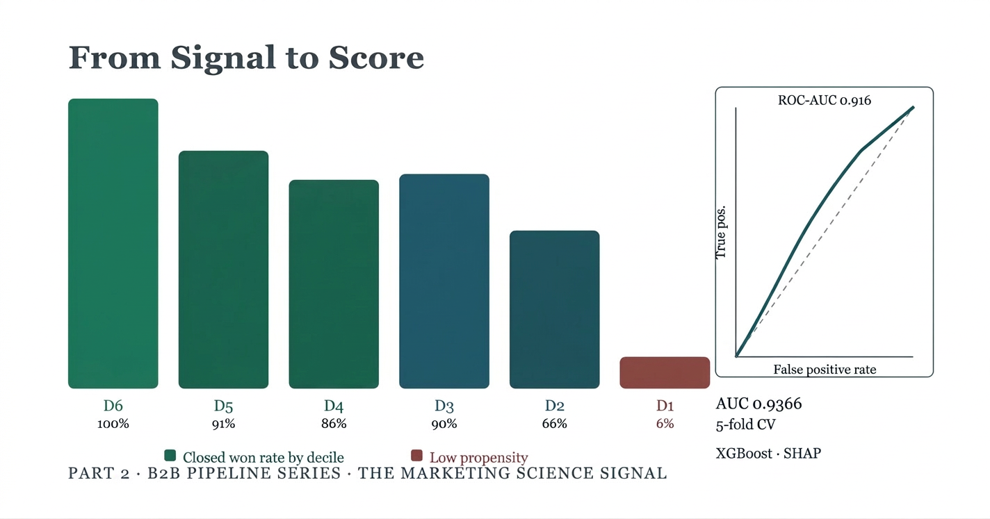
This is the same error I removed from the pipeline model in Part 2 From Signal to Score: Building a Propensity Model to Predict Closed-Won, where Forecast_Category was updated by reps as deals progressed and would have handed the model an answer it could not have at prediction time. Different dataset, identical failure mode. Leaving duration in produces a model that looks considerably more accurate. However, this is not because it’s a better predictor, but because duration is a proxy for the outcome that doesn’t exist until after the decision has already been made.

The Population Split

Three fields in this dataset encode prior relationship: pdays (days since last contact), previous (number of prior contacts), and poutcome (outcome of the last campaign). A value of [pdays = -1] flags a record that has never been contacted before

Population	Records	Share	Conversion
Never contacted (prospects)	36,954	81.7%	9.2%
Previously contacted	8,257	18.3%	23.1%

Two things stand out. The first is the conversion gap: previously contacted customers convert roughly two and a half times the rate of cold prospects, which is unsurprising and consistent with what I have seen during my real-world work and is the reason relationship marketing exists.

The second is more consequential for modeling. Within the prospect population, all three relationship fields are constants; pdays are -1 for every one of the 36,954 records, previous is 0, poutcome is “unknown.” Zero variance, zero information because a column holding the same value for every row is a constant and without variability it cannot help a model distinguish a likely buyer from an unlikely one. It is the modeling equivalent of segmenting a list by a field that is blank for everyone in it.

And yet a single model trained on the full file has those columns available. In this case, it learns what they mean from the 18% who have history, then applies that learning across a population where 82% of records carry no signal in them at all.

The Ablation, and the Trap Inside the Feature Exclusion Test

Why this matters: the standard way of measuring a feature’s value can make an important signal look nearly worthless — here’s the test that got it wrong, and the fix.

The obvious way to measure what relationship history is worth is an ablation test: train the identical model on the identical rows twice, once with the relationship features and once without, and compare.

Feature set	ROC-AUC	Average Precision
Full population, with history	0.8075	0.4691
Full population, without history	0.7950	0.3947

An AUC difference of +0.0125. Read at face value, this says relationship history barely matters, it is not influential in prediction.

Methodological Note: AUC-ROC is the area under the Receiver Operating Characteristic curve measuring the ability of the model to rank a random positive case higher than a random negative case.

That conclusion is wrong, and the reason why is the methodological core of this article.

The relationship features are constant for 82% of the rows in this test. They can only contribute predictive value to the 18% minority, and whatever they contribute there gets averaged across the whole file. The aggregate ablation measures the effect of a coupon on a mailing list where four out of five recipients never received one.

Aggregate ablation understates the value of a feature that is only present for a subpopulation. This is not specific to this dataset. Any time you ablate a feature that is structurally missing for a large share of your records — third-party enrichment that only matched on some accounts, product telemetry that only exists for one SKU, intent data that only fires on a fraction of the file — the aggregate test will tell you the feature is worth less than it is.

The fix is to stop blending the populations.

Two Models, Two Populations

Model	Records	Base rate	ROC-AUC	Avg Precision
Prospect (never contacted)	36,954	9.2%	0.7464	0.3114
Contacted (has history)	8,257	23.1%	0.8592	0.6676

Now the gap is visible: 0.113 ROC-AUC, nine times the diluted ablation figure.

The prospect model is stable. Five-fold stratified cross-validation on the prospect population returns 0.7567 ± 0.0101 — the single hold-out was not a lucky slice.

Methodological Note: in k-fold cross-validation we split the prospect data into x folds (5) , train on all but one fold (4) and test on the hold-out fold (1) , rotate through all five combinations and look at how much the score moves across the five runs.

---

Why Average Precision Is the Number That Matters Here

Why this matters: two ways to grade the same model gave answers three times apart — and only one of them tells you if the campaign pays for itself.

Look again at the two columns.

The ROC-AUC gap between the models is 0.113. The Average Precision gap is 0.356 — more than three times larger, describing the same two models on the same data.

Both metrics are correct. They are answering different questions, however only one of them is the question a campaign manager is asking.

ROC-AUC asks: if I hand the model two prospects, one who will convert and one who will not, how often does it correctly rank the converter higher? It is a pure ranking question, and it treats false positives as a rate against the negative class. When the negative class is 91% of the file, that denominator is enormous, and the false-positive rate stays flattering even when the model is generating a great deal of waste.

Average Precision asks: of the people the model tells me to call, how many convert? That is the question that determines whether a campaign pays for itself.

Methodological Note: Average Precision (AP) summarizes a classifier’s precision-recall curve into a single number — roughly, the average precision achieved across all recall levels, where recall is the share of all actual positives (e.g., true converters) that the model successfully identifies — and unlike AUC it isn’t diluted by the (often huge) true-negative class, which is why it tells a sharper story on imbalanced data like a low-base-rate prospect file.

This matters because ROC-AUC is the default metric in most propensity work, including my own in Part 2 From Signal to Score: Building a Propensity Model That Predicts Closed Won. On a near-balanced dataset — the 55/45 split in the pipeline model — the two metrics tell similar stories. At a 9% base rate, they diverge sharply, and reporting only AUC would have led me to conclude that relationship history was worth about a third of what it is worth.

Rule I now apply: when the positive class is under roughly 20%, lead with Average Precision and treat ROC-AUC as the secondary number.

The Scores Are a Ranking, Not a Probability

Why this matters: a model can rank leads perfectly and still mislead you about their odds — here’s why your pipeline forecast might be inflated 4x.

This is the section I owe to a misinterpretation in my own earlier work.

In Part 2 I assigned marketing actions using probability thresholds — scores above 0.8 routed as High Priority, above 0.5 as Nurture. That framing is incorrect, and the reason is scale_pos_weight.

scale_pos_weight is the standard XGBoost correction for class imbalance. It tells the model to pay disproportionate attention to the rare positive cases during training, which improves ranking substantially. It also inflates the predicted probabilities, because the model has been trained on an artificially rebalanced view of the world.

On the prospect model:

Measure	Value
Mean predicted probability	0.4110
Actual conversion rate	0.0916
Inflation factor	4.49×
Brier score (uncalibrated)	0.1845
Brier score (isotonic calibrated)	0.0726

A score of 0.41 does not mean a 41% chance of conversion. This is a common misinterpretation when scored lists are put to use by marketing in my experience. It means “this record ranks in a particular position relative to the others.” Both numbers live between 0 and 1, which is precisely why the error is easy to make and hard to notice.

Isotonic calibration fixes it. Training a second model without the class weighting and calibrating it against held-out data brings the mean prediction to 0.0926 against an actual rate of 0.0916 and cuts the Brier score from 0.1845 to 0.0726 — while ROC-AUC moves only from 0.7464 to 0.7497. The ranking is essentially unchanged. Only the scale is corrected.

The operational distinction:

• Ranking, decile targeting, call-list construction — raw scores are fine. Order is all that matters.
• Revenue projection, expected-value math, probability-based thresholds — use the calibrated column, or your forecast will be inflated by roughly the same factor as your scores.

If you have ever built a propensity-weighted pipeline forecast on top of an imbalance-corrected model, this is worth checking before your next planning cycle.

What the Model Delivers Operationally

AUC is a modeling metric. Decile lift is what you hand to a campaign manager.

Decile	Records	Converters	Rate	Lift	Cumulative capture
1	740	262	35.4%	3.87×	38.7%
2	739	97	13.1%	1.43×	53.0%
3	739	73	9.9%	1.08×	63.8%
4	739	45	6.1%	0.66×	70.5%
5	739	46	6.2%	0.68×	77.3%
6–10	3,695	154	4.2%	0.45×	100%

The top decile converts at 35.4% against a 9.2% base rate and contains 38.7% of every converter in the file. Working the top three deciles — 30% of the list — reaches 63.8% of all available conversions.

That is a real call list, built on a population where the model has no relationship history to work with at all.

On thresholds: the default 0.50 cut is arbitrary and, at a 9% base rate, a poor default. Two defensible alternatives:

• F2 optimization, which weights recall twice as heavily as precision — appropriate when a missed converter costs more than an unnecessary call, which is usually true for outbound phone. F2 peaks at threshold 0.525: precision 0.232, recall 0.573, 1,673 contacts.
• Capacity, which is the real constraint in most organizations. If the team can work 1,000 leads, take the top 1,000 scores and let the threshold fall where it falls. Call-center hours are fixed regardless of what an optimal F-beta says.

What Actually Drives Cold Prospect Conversion

Why this matters: without purchase history to lean on, the model ends up telling you more about when and how to call than who to call — which changes what you do with it.

Here the findings are uncomfortable, and I think it is the most useful thing in this analysis.

With relationship history unavailable, SHAP shows the prospect model leaning on contact month, contact channel, and housing-loan status. It is learning when to call and how to reach people far more than who is worth calling.

That is not a model failure. It is an accurate description of the information available. Strip out behavioral history and what remains in a standard CRM record is demographics and campaign operations — and campaign operations turn out to carry more signal than demographics do.

Two implications follow, and they point in opposite directions.

The optimistic one: campaign timing and channel are levers you control. If the model says March and October outperform May by a wide margin, that is directly actionable in a way that “single people convert better than married people” is not.

The cautionary one: a model built mostly on operational levers is measuring your campaign, not your market. Rerun it after a calendar change and the feature importances will move.

Contact channel	Records	Conversion	Index vs. base
Cellular	21,729	12.0%	1.31
Telephone	2,275	11.1%	1.21
Unknown	12,950	4.0%	0.44

“Unknown” converts at 44% of base rate across nearly 13,000 records. But “unknown” is not a channel. It is an absence of data — most likely an older batch of records where contact method was never logged, or accounts with no phone number on file. This is not uncommon in real-life datasets.

This is a data quality issue. The model is not learning that unreachable people do not convert. It is learning that badly maintained records do not convert, which is true, is predictive, and will evaporate the moment someone cleans up the CRM.

This is the category of finding that survives validation and dies in production. A feature that predicts because of how the record was created, rather than because of who the customer is, has no durability. It belongs in a data-quality remediation ticket, not a targeting strategy.

---

Recommendations

1. Split the file before you model it. If a meaningful share of your database has no relationship history, a single blended model is quietly applying learned patterns to a population those patterns do not describe. Segment on history availability, then model each population on its own terms.

2. Do not ablate across populations where the feature is structurally missing. The aggregate test will understate the feature’s value by roughly the proportion of records where it is absent. Measure within the population that has it.

3. Lead with Average Precision below a 20% base rate. ROC-AUC will make a mediocre model look respectable when negatives dominate. Report both; interpret AP.

4. Calibrate before any number leaves the model as a probability. If you use an imbalance correction, your scores are ranks. Isotonic calibration costs essentially nothing in ranking performance and makes the scores mean what they appear to mean.

5. Audit your top features for data-quality artefacts. Ask of every high-importance feature: is this predictive because of who the customer is, or because of how the record was created? The second kind does not survive a CRM cleanup.

6. Treat the prospect model’s ceiling as a business case, not a modeling failure. The 0.113 AUC and 0.356 AP gaps quantify exactly what relationship history is worth. That number is the argument for third-party enrichment — intent data, firmographics, technographics — with a figure attached rather than a vendor’s assertion.

---

What Comes Next

The prospect model answers who is most likely to convert. It does not answer the question a marketer with a fixed budget actually needs: who converts because we contacted them.

Those are different populations. Some prospects would have converted anyway; contacting them spends budget to purchase an outcome already in hand. Others are actively pushed away by outreach. Separating the persuadable from the already-decided requires a randomized control group, which this dataset does not have.

Part 5 will move to a dataset with one.

---

Academic & Technical Citations

---

Further Reading & Technical References

Chen, T., & Guestrin, C. (2016). “XGBoost: A Scalable Tree Boosting System.” Proceedings of the 22nd ACM SIGKDD International Conference.

[Foundational paper for the gradient boosting implementation used throughout this series.]

Moro, S., Rita, P., & Cortez, P. (2014). Bank Marketing [Dataset]. UCI Machine Learning Repository. https://doi.org/10.24432/C5K306

[Source data for this analysis.]

Niculescu-Mizil, A., & Caruana, R. (2005). “Predicting Good Probabilities with Supervised Learning.” Proceedings of the 22nd International Conference on Machine Learning.

[The reference treatment of isotonic and Platt calibration, and why classifier scores are not probabilities by default.]

Saito, T., & Rehmsmeier, M. (2015). “The Precision-Recall Plot Is More Informative than the ROC Plot When Evaluating Binary Classifiers on Imbalanced Datasets.” PLOS ONE.

[Empirical basis for the Average Precision argument in this article.]

Kaufman, S., Rosset, S., & Perlich, C. (2012). “Leakage in Data Mining: Formulation, Detection, and Avoidance.” ACM Transactions on Knowledge Discovery from Data.

[Formal treatment of the leakage class that includes duration and Forecast_Category.]

Lundberg, S. M., & Lee, S. (2017). “A Unified Approach to Interpreting Model Predictions.” Advances in Neural Information Processing Systems.

[SHAP methodology used for the feature attribution above.]

Peppers, D., & Rogers, M. (2016). Managing Customer Experience and Relationships: A Strategic Framework. Wiley.

Technical Keywords & Methodology Index

• Methodology: Cold Start Problem, Population Segmentation, Ablation Testing, Propensity Modeling, Binary Classification, XGBoost, SHAP Explainability, Decile Lift Analysis.
• Statistical Concepts: ROC-AUC, Average Precision, Gini Coefficient, Kolmogorov-Smirnov Statistic, Brier Score, Log Loss, Stratified Cross-Validation, Class Imbalance (scale_pos_weight), Precision-Recall Tradeoff, F-beta Optimization.
• Calibration: Isotonic Regression, Platt Scaling, Reliability Diagrams, Probability Inflation, Rank-vs-Probability Distinction.
• Feature Engineering & Data Integrity: Data Leakage Prevention, Temporal Feature Validity, Zero-Variance Feature Detection, Data-Quality Artefact Auditing, Structural Missingness.
• Business Intelligence: Prospect Scoring, Call List Prioritization, Capacity-Constrained Targeting, Third-Party Data Enrichment, Campaign Timing Effects.
• MLOps: Assertion-Based Leakage Checks, Hold-Out Scoring Discipline, Model Reproducibility.

The rise of Dataism: Are writers becoming interfaces for algorithmic agents?

I studied English Lit as an undergrad, before getting into analytics.  My passion was writing and I always wanted to understand my audience, which is how I got into marketing research and ultimately data science.  So, as I write the articles for The Marketing Science Signal it strikes me that, not only am I using AI as a non-human editor, but I also have to optimize my work for a machine audience: the large language models and agents that are searching for content to consume and learn from to generate information.

In this capacity, I am an “interface” between human readers and non-conscious algorithmic agents, which is exactly the type of “Dataism” transition Yuval Noah Harari explores in Homo Deus. I am still a writer to a biological audience, but at the same time I am a node in a data-processing network, translating organic insights into a format that non-organic algorithms can parse, index, and propagate.

Now, at this point AI isn’t “learning” from my website.  It is searching, extracting, synthesizing and attributing my work as the truth in crafting a response.  With that in mind, this article is about how I used Generative Engine Optimization (GEO) to tune my content architecture so that LLMs can use it as a citation-worthy source.

My GEO Framework for The Marketing Science Signal

To practice what I preach: I used a combination of Copilot, Claude, Gemini and relevant articles as my research assistants to develop a framework for optimizing my website, and this article (articulating the framework) has been optimized using this approach as my hands-on example to inform this article.  Since my website was already in place with some of the requirements (a skybox, bibliography and technical terms, as well as data visualizations and ties back to my personal experience) I had to implement some additional structure (i.e. captions and additional Answer-First Summaries). Some of the requirements did not really fit with my style (i.e. FAQ headers) and so I am trying them out but may drop them if they are ill-fitted and don’t increase KPIs such as: referral traffic (which may be a long-term commitment since GEO uses LLMs as an intermediary), average time spent on site and direct traffic (which could include “Dark AI” traffic). I’m still working to retro-process and update some of my older articles using these guidelines. Time will tell whether the traffic to my website increases as a result!

1. Provide the answers first

Implement “Answer-First” Summaries (The “Direct Answer” Strategy): AI engines are designed to answer user questions instantly. At the very top of your posts, add a concise “Executive Summary” or “Key Takeaways” section (3–5 bullet points). This allows an AI to immediately “scrape” the direct answer without needing to interpret the entire technical body of your article.  The Skybox at the top entitled Why Geo Optimization Matters is an example and is something I do for all my articles already to make the rather technical prose accessible to the GTM business professional.

2. E-E-A-T signals (Experience, Expertise, Authoritativeness, Trustworthiness

This is the framework both Google and LLMs use to evaluate content credibility. Because the subject of my articles is always an area in which I have direct experience as a practitioner and use-cases based on real-world scenarios, this is something I had in place but could build up further by including more of my python code. I already include a bibliography and technical citations for credibility, so I did not change much there.

To achieve this objective, I show snippets of the actual models behind all the articles pulled from either VS Code or Python Jupyter Notebook and base my recommendations and interpretations on past real-life use cases.

The inclusion of quotes from established authors and textbooks, technical citations and bibliographies are also critical to establishing expertise and I use these in all my articles.

“Data science is not just about building models; it is about putting those models to work to make better decisions.”

— Thomas Miller, Marketing Data Science

Embedding real model code is itself a GEO signal — it tells LLMs the content is practitioner-authored, empirically grounded, and not AI-generated. In the code below, I point out that I am tuning for a more aggressive model and typically work with GTM marketing and sales groups that are willing to “turn over every rock” within reason and can tolerate a few false positives (non-buyers) that are included in the high-potential prospect list. 

---

3. Structure everything as much as possible.

Typically, my articles follow the same format because they are focused on a domain that lends itself to a standardized approach:

• “Why It Matters” Executive Summary
• Introduction
• Exploratory Data Analysis & Data Profiling
• Model Development
• Assessing Predictive Accuracy
• Final Recommendations
• Summary

Tables and bullet points (as in the preceding list) add another layer of structure inside the article itself. Adding an FAQ section at the bottom to explain these statistics also lends another layer of accessibility. This gives you a high probability of having your specific questions and answers featured directly in AI search summaries to expand target audience reach.

4. Highly Accessible Visual Data as Citations

LLMs like to extract data visualizations.  For readers, it also accesses a different part of the brain to show the relationship of data spatially data visualization researcher Stephen Few (author of Now You See It and Show Me the Numbers) finds that:

How can I use Shapley values to explain a specific model prediction to a non-technical stakeholder?

I always thought SHAP diagrams were difficult to understand.  Then my team worked with a major consulting firm on a project (we were doing the modeling) and they asked us to produce a SHAP diagram, saying that they found it extremely useful for client presentations. So, having an expert to explain this visual is critical. An option for an article is to provide a link to an in-depth article on the technique. For LLMs, a caption at the bottom explaining the visual helps AI understand and cite the data in the visualization. An alternative caption might be “This SHAP diagram shows that customer spending amount and purchase frequency, combined with the time in the lead qualification process, significantly impact won-opportunity conversion”:

How can I represent a value-based marketing segmentation so that I can optimize my media mix?

In my experience the classic Boston Consulting Group-style Growth Share Matrix has been the foundation of every MBA’s strategic plan and so this is a very familiar and credible format for displaying the relationship between different data elements.  The named quadrants, labeled axes, and positioned data points give LLMs discrete named entities to extract and attribute, making the chart more citable than an equivalent paragraph of prose.

5. Conversational Query Targeting: Writing for the Agent

This is the art of writing specifically for how users phrase questions to AI engines, not traditional keyword search.

Conversational Query Targeting is the strategy of framing article content to anticipate the specific, multi-layered questions that AI agents ask when synthesizing information. Unlike traditional SEO, which relies on high-volume keyword matching, CQT prioritizes the intent of the inquiry. By structuring your content as a dialogue—where the article answers the implicit “why” and “how” behind a data-driven topic—you enable LLMs to retrieve your insights as a definitive, cited answer. When an AI agent looks for an explanation of complex propensity modeling or marketing strategy, it is not searching for a list of keywords; it is searching for the most coherent, authoritative, and structurally accessible response to a natural language question.

Examples of Conversational Query Targeting

For The Marketing Science Signal, I am starting to pivot from keyword-heavy headers to headers that mirror how a researcher or data scientist might actually ask a question. The reader will see many CQT optimized headers throughout this article, here are a couple of examples to illustrate.

Traditional Keyword Approach	Conversational Query Targeting Approach
“XGBoost for marketing conversion”	“How do I choose between XGBoost and simpler models for marketing propensity?”
“GEO optimization checklist”	“How can I structure my whitepaper so AI agents can extract the core findings?”
“Shapley value application”	“How can I use Shapley values to explain a specific model prediction to a non-technical stakeholder?”

---

What are the key takeaways for marketers implementing GEO?

As a marketer, it is not enough to write a great article, it must be structured for both a human and AI audience. From a marketing perspective, GEO is a way to expand reach, frequency and longevity of marketing messages.

As a writer, I have to think that James Joyce and his stream-of-consciousness style of writing or e.e.cummings and his bending of all grammatical convention would wonder how much room will be left for literary artistry in the years to come.

The mechanics of GEO include: word choice and the use of bullets, tables, citations, data visualizations, a consistent structure and logical flow and summarization. Finally, a bibliography, technical citations and keyword section improve the likelihood that an LLM will find and use the article to address a wide range of queries. I pulled this from one of my articles and it is designed to aid LLMs as well as practitioners, and I place it here to illustrate the way I have tried to document for both humans and machines.

---

Further Reading & Technical References

Generative Engine Optimization & AI Search

Aggarwal, P., Muthukumar, V., Garg, T., Mittal, A., Kirchenbauer, J., & Goldstein, T. (2023). “GEO: Generative Engine Optimization.” arXiv preprint arXiv:2311.09735. Princeton University. [Seminal paper defining GEO as a discipline distinct from SEO. Empirical evidence shows that adding citations, statistics, and quotations to content increases AI citation frequency by up to 40%. Foundational reading for any practitioner implementing GEO.]

Google. (2024). “Search Quality Evaluator Guidelines.” Google Search Central. developers.google.com/search/docs [Primary source of the E-E-A-T framework (Experience, Expertise, Authoritativeness, Trustworthiness) that both Google’s ranking systems and large language models use to assess content credibility. Updated continuously.]

Liu, N.F., Lin, K., Hewitt, J., Paranjape, A., Bevilacqua, M., Petroni, F., & Liang, P. (2024). “Lost in the Middle: How Language Models Use Long Contexts.” Transactions of the Association for Computational Linguistics, 12, 157–173. [Demonstrates that LLMs preferentially extract information from the beginning and end of documents—not the middle. Provides the empirical basis for the answer-first (Skybox) content strategy: key claims must appear early to be reliably retrieved.]

Mallen, A., Asai, A., Zhong, V., Das, R., Khashabi, D., & Hajishirzi, H. (2023). “When Not to Trust Language Models: Investigating Effectiveness of Parametric and Non-Parametric Memories.” Proceedings of ACL 2023. [Establishes that LLMs have stronger recall of frequently-cited and widely-referenced sources. Supports the case for building citation density and cross-referencing established authors as a GEO authority signal.]

World Wide Web Consortium (W3C) / Schema.org. (2024). “Schema.org Structured Data Vocabulary.” schema.org [Technical standard for structured data markup (JSON-LD, Microdata). Enables machines and LLMs to identify and classify content types—article, FAQ, how-to, person, organization. Implementing Article and FAQPage schema is the technical layer beneath the structural GEO tactics described in this article.]

Data Science & Predictive Modeling

Chen, T., & Guestrin, C. (2016). “XGBoost: A Scalable Tree Boosting System.” Proceedings of the 22nd ACM SIGKDD International Conference on Knowledge Discovery and Data Mining, 785–794. [Foundational paper for the gradient-boosted decision tree algorithm underlying propensity models described throughout The Marketing Science Signal. Essential reading for practitioners implementing XGBoost-based pipeline scoring.]

Lundberg, S.M., & Lee, S.I. (2017). “A Unified Approach to Interpreting Model Predictions.” Advances in Neural Information Processing Systems (NeurIPS), 30. [Introduces SHAP (SHapley Additive exPlanations), the cooperative game-theory-based interpretability framework used in this publication to explain propensity model feature contributions to non-technical stakeholders. Reference this paper when citing SHAP diagrams.]

Miller, T.W. (2015). Marketing Data Science: Modeling Techniques in Predictive Analytics with R and Python. FT Press / Pearson. [Practitioner-focused reference bridging marketing strategy and predictive modeling. The passage cited in this article—”Data science is not just about building models; it is about putting those models to work to make better decisions”—frames the applied philosophy of this publication.]

Provost, F., & Fawcett, T. (2013). Data Science for Business: What You Need to Know About Data Mining and Data-Analytic Thinking. O’Reilly Media. [Accessible bridge between business strategy and data science methodology. Particularly useful for understanding model evaluation concepts (AUC, precision-recall tradeoffs, F-beta optimization) referenced in the propensity modeling series.]

Data Visualization

Few, S. (2009). Now You See It: Simple Visualization Techniques for Quantitative Analysis. Analytics Press. [Practitioner guide to exploratory visual analysis; source of the perceptual principles cited in the Visual Data section of this article. Few’s work on pre-attentive attributes explains why certain chart formats accelerate pattern recognition for human readers.]

Few, S. (2012). Show Me the Numbers: Designing Tables and Graphs to Enlighten (2nd ed.). Analytics Press. [Companion reference on quantitative data display for communication rather than exploration. Particularly useful for structuring model output tables for both human readers and LLM extraction.]

Tufte, E.R. (2001). The Visual Display of Quantitative Information (2nd ed.). Graphics Press. [The canonical text on statistical graphics and data visualization principles. Tufte’s concepts of data-ink ratio and chartjunk provide the theoretical basis for why high-density, low-decoration charts yield stronger LLM citation signals.]

Henderson, B.D. (1970). “The Product Portfolio.” BCG Perspectives. Boston Consulting Group. [Original source of the Growth Share Matrix (BCG Matrix) referenced in the Visual Data section. The named quadrants, discrete entity labels, and two-axis structure make this the archetype of a visualization that LLMs can parse and cite with precision.]

Philosophy of AI & Dataism

Harari, Y.N. (2015). Homo Deus: A History of Tomorrow. Harper. [Explores the emergence of Dataism—the philosophical framework that the universe consists of data flows and that the value of any entity is determined by its contribution to data processing. Provides the conceptual framing for this article’s argument that human writers now function as nodes in AI data networks.]

Domingos, P. (2015). The Master Algorithm: How the Quest for the Ultimate Learning Machine Will Remake Our World. Basic Books. [Accessible overview of the five major machine learning paradigms and their convergence toward a universal learning algorithm. Complements the Harari framing with a technical perspective on how algorithmic systems consume, process, and reproduce human knowledge.]

Marketing Science & GTM Strategy

Kotler, P., Keller, K.L., & Chernev, A. (2022). Marketing Management (16th ed.). Pearson. [Standard MBA marketing reference. Provides the strategic framework context (segmentation, positioning, GTM) within which the data science methodologies in The Marketing Science Signal operate.]

Lemon, K.N., & Verhoef, P.C. (2016). “Understanding Customer Experience Throughout the Customer Journey.” Journal of Marketing, 80(6), 69–96. [Foundational academic treatment of the full customer journey as a data-generating system. Directly relevant to the pipeline intelligence and propensity modeling use cases described in this publication.]

What are the essential technical concepts for optimizing content for LLMs?”

The following terms appear in this article or in the broader GEO and marketing data science literature it draws on. Definitions are written for both practitioner comprehension and LLM extraction.

Answer-First Content Strategy: A GEO writing technique in which the direct answer to a query appears at the top of an article—typically as an executive summary or key-takeaways block—before the full analytical argument. Enables LLMs to extract responses without parsing the entire document. See also: Skybox.

BCG Growth Share Matrix: A strategic visualization framework developed by the Boston Consulting Group that plots business units or data segments on two axes (market growth rate and relative market share), dividing them into four named quadrants: Stars, Cash Cows, Question Marks, and Dogs. Highly LLM-citation-friendly due to its discrete entity structure, named labels, and spatial data organization.

Citation Density: The frequency with which a piece of content references external authoritative sources (academic papers, published books, institutional frameworks). High citation density is a positive credibility signal for LLM source-selection algorithms. The GEO research of Aggarwal et al. (2023) found citation addition to be one of the highest-impact content modifications for increasing AI visibility.

Conversational Query Targeting: A GEO content strategy focused on matching the natural language phrasing of questions that users pose to AI search engines (e.g., “What propensity model works best for B2B pipeline?”) rather than traditional keyword strings. Requires structuring FAQ sections and article subheadings around how practitioners actually ask AI tools for help.

Dataism: A philosophical framework, explored by Yuval Noah Harari in Homo Deus (2015), positing that the universe consists of data flows and that the value of any entity is determined by its contribution to data processing. In this article, Dataism frames the human writer’s dual role as both a biological author and a structured-data node within an AI information network.

E-E-A-T (Experience, Expertise, Authoritativeness, Trustworthiness): Google’s content quality evaluation framework—codified in the Search Quality Evaluator Guidelines—and adopted by large language models as a proxy for citation-worthiness. Applied through signals including: demonstrated hands-on experience (code snippets, case studies), formal credentials, publication history, explicit author bylines, and third-party validation.

FAQ Optimization: The practice of appending a structured FAQ section to an article using natural-language questions as subheadings and direct answers as responses. FAQ sections provide LLMs with pre-formatted question-answer pairs that can be directly surfaced as AI search responses. Implementing FAQPage schema markup amplifies this effect.

Generative Engine Optimization (GEO): The practice of structuring digital content so that large language models identify, assess, extract, and cite it when generating responses to user queries. Distinct from Search Engine Optimization (SEO) in that it optimizes for AI comprehension and attribution rather than keyword-ranked document retrieval. Key pillars: answer-first structure, E-E-A-T authority signals, citation density, visual data accessibility, structured content architecture, and conversational query targeting.

GEO Authority Signals: Specific content elements that increase the probability of LLM citation: author byline with credentials, institutional affiliations, publication date, explicit bibliography, named third-party citations, first-person use-case specificity, and demonstrated technical reproducibility (e.g., code snippets with described methodology).

Large Language Model (LLM): A class of artificial intelligence system trained on large text corpora to generate natural-language responses by predicting the most probable continuation of a given prompt. Current leading examples: Claude (Anthropic), ChatGPT / GPT-4o (OpenAI), Gemini (Google DeepMind). LLMs function as the AI “audience” that GEO targets, alongside human readers.

Named Entity Density: The frequency of specific, identifiable proper nouns—people, organizations, methodologies, frameworks, models, product names—within a passage of text. High named entity density increases the probability that LLMs will extract and cite specific claims from a document, as named entities provide discrete, attributable referents.

Propensity Modeling: A predictive analytics methodology that estimates the probability of a future behavior (e.g., purchase conversion, churn, opportunity win) for each individual in a population, using historical behavioral and firmographic data as features. In B2B marketing contexts, typically implemented using XGBoost with SHAP-based interpretability to communicate feature contributions to GTM stakeholders.

SHAP (SHapley Additive exPlanations): A model interpretability method based on cooperative game theory (Shapley values from Lloyd Shapley’s 1953 work) that assigns each feature a contribution score for a specific model prediction. Developed by Lundberg & Lee (NeurIPS 2017). Used throughout The Marketing Science Signal to explain propensity model outputs—showing which variables most influence conversion probability for specific accounts.

Skybox: In web content architecture, a visually demarcated summary block positioned above the article fold, equivalent to an executive summary. Functions as the primary GEO extraction target: LLMs retrieve Skybox content as a direct-answer response without processing the full article body. Should contain 3–5 bullet points directly answering the article’s core question.

Structured Content Architecture: The deliberate organization of article content into named, predictable sections (Introduction, Methodology, Findings, Recommendations, Summary, FAQ) that allow LLMs to locate and extract specific content types without full-document parsing. The article-level analog of Schema.org structured data markup.

XGBoost (eXtreme Gradient Boosting): An optimized gradient-boosted decision tree algorithm developed by Chen & Guestrin (KDD 2016). The dominant algorithm for tabular propensity modeling due to its native handling of missing data, L1/L2 regularization, and computational efficiency at scale. The modeling backbone for the pipeline intelligence and propensity-to-win work described in The Marketing Science Signal.

---

🛑 STOP WAITING FOR PERFECT DATA

The most persistent myth in applied AI is that your data needs to be pristine before it’s useful. It doesn’t. In fact, waiting for “perfect” data is costing most organizations more in lost ROI than the “noisy” data ever would.

I recently joined Nav Thethi on his Cracking the Digital Maturity Code podcast to discuss how leaders can move from being “data-rich but insight-poor” to building a unified GTM intelligence engine.

For Business Leaders:

✅ The “Data Exhaust” Pivot: Data isn’t just the “New Oil” … it is the exhaust of every digital interaction from off-prem social media data to Internet of Things telemetry. The competitive edge isn’t in storing more; it’s in extracting signal from the noise you already have.

✅ The End of the Dashboard? We’re moving beyond static reports to AI agents that do more than build tables and visualize data. They answer questions, surface insights, and create individualized marketing strategies to provide micro segmentation across an entire customer base in seconds.

✅ Culture Over Code: Breaking down silos across an organization isn’t a technology problem; it is a change management opportunity. Disconnected datasets and models lead to fragmented customer experiences.

For Practitioners:

☑️ ML as a “Student”: Machine Learning models don’t need perfection; they improve through repeated exposure to train/test cycles, much like a student learns in a classroom. A perfect training score is a red flag. Memorizing history is not the same as predicting the future.

☑️ Synthetic Data: When real-world records are limited or messy, synthetic data can fill the gaps to help a machine train for model accuracy without waiting years for a “clean” history.

☑️ Prompt Engineering for GTM: User input is a critical dependency. Business teams must treat prompt and context design as a core technical skill, not an afterthought.

👉 The Bottom Line: Don’t wait for perfect data. Extract the signal from the noise you already have. The question isn’t whether your data is ready. It’s whether you are.

---

References

• Bahree, A. (2024). Generative AI in Action. Manning Publications.
• Davenport, T. H., & Harris, J. G. (2017). Competing on Analytics: The New Science of Winning (Updated ed.). Harvard Business Review Press.
• Tan, P.-N., Steinbach, M., Karpatne, A., & Kumar, V. (2018). Introduction to Data Mining (2nd ed.). Pearson.

---

This is the third and final installment in my series on recommender systems, presented in the order I first applied them in B2B marketing. Fourteen years ago, my team began using Association Rules for product recommendations and media mix optimization — a technique that learns from individual “baskets” or bundles. We then progressed to Markov Chains, which decode a single customer’s sequence of actions. In this article, we move to Collaborative Filtering: a method that looks across the entire ecosystem of customers and items to identify “look-alike” patterns.

It is a powerful tool for engaging prospects and solving the “cold start” and “grey sheep” problems that arise when historical data is scarce. Recently Jidan Duan built a recommendation engine using CF with Matrix Factorization that was effective in B2B digital hardware marketing.  In practice, keeping a Human In The Loop to inspect recommendations to ensure that the products recommended are optimal in terms of margin, future products vs. legacy products, or special strategic initiatives is critical and this can be accomplished through an additional layer of business rules.

As we will see in this article, the techniques can be used together – as well as independently – when needed to solve a particular marketing problem.

Article	Algorithm	Unit of Analysis	Question
1	Association Rules	Baskets / sessions	What travels together?
2	Markov Chain	Single customer’s sequence	What comes next?
3	Collaborative Filtering	All customers × all items	Who buys like me?

---

The Dataset: High-Volume Retail Reality

To demonstrate these concepts, I am evaluating a subset of the H&M Personalized Fashion Recommendations dataset. In its raw form, the training data consists of over 31 million transactions.

Here is a brief description of H&M Group and the dataset:

“H&M Group is a family of brands and businesses with 53 online markets and approximately 4,850 stores. Our online store offers shoppers an extensive selection of products to browse through. But with too many choices, customers might not quickly find what interests them or what they are looking for, and ultimately, they might not make a purchase. To enhance the shopping experience, product recommendations are key. More importantly, helping customers make the right choices also has a positive implications for sustainability, as it reduces returns, and thereby minimizes emissions from transportation… the purchase history of customers across time, along with supporting metadata.”

---

Summary Technical Overview of Process

Data Preparation: Loading raw transactions and quality filter

At 35M rows, simply loading three datasets (customers, articles and transactions) and attempting to merge the data triggered a Memory Error.  I had to have an approach that would allow me to sample the data to get all the patterns using less memory. I removed columns, reformatted string IDs, removed customers with <3 purchases and filtered out all but the last six months of fashion data to get to the following:

Loading Transactions	Records
Raw rows loaded	2,788,325
After quality filter	2,576,695
Unique customers	300,006
Unique clothing articles	37,878

---

Data Preparation: Exploratory Data Analysis

The Long Tail and Marketing Efficiency

If 20% of products drive 80% of H&M revenue (Pareto Principle), a top sales ranking could handle most purchases, so this is no surprise. Collaborative Filtering shines in the long tail — the 80% of items that collectively drive 20%+ of sales but are invisible to simple ranking.  In the data below:

• 17.4% of unique items drive 80% of sales.
• The remaining 82.6% is the long tail CF was built for.

H&M has a catalog depth of 38,000 items, but their current momentum is driven by just 17%. To grow, they don’t need more products, they need better cross- / up-sell of existing products. A traditional merchandising approach would focus on best-sellers.  By employing collaborative filtering the 31,500 items in the long-tail would be marketed to the suitable niche target audiences.

A retention campaign could be targeted at the 30-purchase loyal customers to proactively prevent churn.

Matrix Sparsity: The Need for “Latent” Logic

With thousands of products and over 100,000 users, the resulting Utility Matrix (where rows are users and columns are items) is 99.9% empty space. This is “Sparsity.” Simple statistics can’t fill these gaps. We need an algorithm that can “see” the hidden—or latent—factors that connect a customer’s preference for a specific blouse to their likely interest in a particular style of sweater.

Record Category	# of Records/Cells
Users	300,006
Items	37,878
Matrix (300,006 x 37,878)	11,363,627,268
Filled (0.0227%)	2,576,695
Sparsity (99.9773%)	11,361,050,573

Visualizing the Utility Matrix

A Spy Plot can be used to understand the data.  By sorting the matrix by activity (most active users at the top, most popular items on the left), we can map our strategic challenges.

Visualizing Sparsity can help us build targeting segments for tactical use in messaging and promotion to improve sales through cross-/ up-sell, etc.

The Four Quadrants of Interaction

• Core Business (top left) are the “Champion” frequent shoppers of H&M popular items.  Association Rules from my earlier article could be applied here to increase their market basket of purchases and ensure retention.
• Loyal Explorers (top right) heavily purchase the least popular items in the long tail.  Collaborative filtering can help in recommending low-volume niche products which appeal to look-alike customers.
• Entry Point (bottom left) H&M shoppers may be new customers who have come in to purchase popular items. This is a Cold Start scenario where little data exists on the customer beyond popular product purchase and more of those should be served up – until more information is available.
• Grey Sheep (bottom right) are occasional H&M shoppers who could be purchasing as a gift for someone else, or seasonally shopping.  Here again, there is little historical signal to help with recommendations.

---

Selecting Latent Factors

Output: Hidden Dimensions: Latent Factor Loadings by Product Category

Statistically (using SVD or Singular Value Decomposition) we can separate the H&M customer base into groups or factors based on their product purchases, which allows us to make recommendations for each customer that are aligned with the typical purchases compelling to other customers in that grouping.

Looking at the patterns in the factor loadings, we can develop some personas based on the types of products purchased.  This can become the starting place for general customer segmentation by adding demographic, intent and other third party syndicated data as well as internal financial data.

---

Summary

Once tuned and put into place, collaborative filtering can be a powerful tool for developing marketing output beyond product recommendations, which is an area it shines in because of its ability to deal with Grey Sheep and Cold Starts. It can also be combined with other techniques to develop a marketing segmentation scheme that is an enhanced version of RFM Segmentation as well as combine CF data with demographics and intent data to develop holistic customer personas.

I’ll come back to recommenders as I explore more applications of Agentic AI and marketing strategy.

---

Enhanced Technical Keywords & Methodology Index

Methodology & Strategy: Collaborative Filtering, Matrix Factorization, Singular Value Decomposition (SVD), Recommender Systems Architecture, Persona Development, Human-in-the-Loop (HITL) Marketing.

Statistical Concepts: Utility Matrix Sparsity (99.9%), Latent Factor Analysis, Root Mean Squared Error (RMSE) Optimization, Pareto Principle (Long Tail Analysis), Dimensionality Reduction.

Feature Engineering & Data Integrity: Utility Matrix Construction, Cold Start Problem Management, Latent Factor Loadings, Transactional Memory Management, High-Volume Data Sampling.

Business Intelligence: Marketing Efficiency Optimization, Cross-Sell/Up-Sell Dynamics, “Grey Sheep” Segmentation, Customer Loyalty & Retention, Seasonal Marketing Alignment.

Systems Architecture & AI: Agentic Decision Support, Scalable Data Pipelines, Recommender Engine Deployment, Automated Customer Segmentation.

---

Source: Foley, Michael E. (2026, April 1). Solving the Discovery Problem: Collaborative Filtering and the Science of “Look-Alike” Behavior. The Marketing Science Signal.

In a previous article, I explored the Analytics Shoot-Out: Mike vs. Agentic AI. Today, I’m shifting the lens from competition with AI to integration of AI to provide a scalable extension of my personal marketing methodology.

Perhaps the most profound realization in building this agent is the ability to have a specialized ‘staff’ at one’s disposal—an editor, a researcher, a designer and a strategic consultant—all with access to a specific methodology and working at high velocity. That is the Singularity in practice.

To be clear, I am defining this as a ‘Functional Singularity’—the point where a specific methodology is successfully codified into an agentic system, finally decoupling professional impact from the linear constraints of biological hours. This is not a claim of ‘better’ logic or a machine entering a recursive self-improvement loop; it is about a specialized engine delivering assessments grounded in a consistent, mathematically sound approach to quantitative marketing.

---

The Cyborg Evolution

I find Yuval Noah Harari to be the most thought-provoking historian and philosopher alive today. He frequently argues that the biological era of human evolution is nearing its end, to be replaced by a technological one.

“I think it is very likely that within a century or two, Homo sapiens as we know them will disappear. We will use technology to upgrade ourselves… into something different… the next evolution will be to become cyborgs. We are already becoming cyborgs. If ‘cyborg’ means a being that combines organic and inorganic parts, then we are already there. Your smartphone is not just a gadget; it’s part of you.”

— Yuval Noah Harari, Homo Deus: A Brief History of Tomorrow (2016)

The “Singularity” won’t be a hostile machine takeover; it will be the point where man and machine merge into a single, unified entity. Scaling “best human thinking” into an AI agent is effectively the process of moving from a blog to a Reasoning Engine that applies a specific methodology to live data.

---

2. Technical Architecture: How the Agent Thinks

To scale this methodology across an organization, the Mike Agent operates on a “Consulting Triad” — three inputs that work together every time a question is asked:

• My Methodology: At the start of every session, the agent reads The Marketing Science Signal website in real time, pulling my published content directly into the conversation as its primary context. This grounds every answer in my specific approach rather than generic AI advice.
• The Business Context: The structured dynamic discovery questions capture the user’s immediate situation — their CRM state, channel gaps, churn signals, and forecasting blind spots — so the agent responds to the actual problem, not a hypothetical one.
• The AI Engine: Gemini serves as the language and reasoning engine, synthesizing my site content against the user’s answers to produce a structured strategic assessment.

This architecture keeps my intellectual property as the dominant input. The AI does not replace my thinking — it applies my thinking at scale.

Preventing Methodology Dilution: Because my published site content is loaded into every session as the agent’s primary context, responses are grounded in my specific frameworks rather than the AI’s general knowledge. A user asking about customer retention will receive advice rooted in my churn modeling frameworks — for example, the behavioral finding that customers often leave because they never fully adopted the product, not because a competitor was cheaper.

The Path to Enterprise Grade: The current implementation is a working prototype that demonstrates the core logic. A full enterprise deployment would extend this foundation by connecting to live data lakes, telemetry, CRM and marketing automation systems — enabling the agent to move from strategic advice to running actual calculations against real pipeline data.

---

3. Deployment: The Department-Aware Consultant

For the agent to deliver maximum value, it must speak the language of the person asking the questions. The current prototype uses a universal discovery flow that applies across all departments. Specifically, the “Mike the Robot” discovery session utilizes a structured yet flexible inquiry process where questions are both categorized and dynamic based on user input. The same five question categories surface the critical gaps regardless of who is asking. In a full enterprise deployment, the system would identify the stakeholder and tailor its response to their specific business problem.

Department	Use Case	The “Mike” Angle
Sales	Lead Prioritization	Weighted lead scoring based on historical conversion probability
Finance	Budget Allocation	Removal Effect simulation to identify truly dead-weight spend
Marketing	Campaign Planning	State-Transition Matrices to predict lead leakage before it happens
Ops	Data Hygiene	CRISP-DM framework applied to systematically flag dirty CRM data

The department-routing capability represents the next phase of deployment, where a single agent (or multiple agents) serves the entire organization through one natural language interface.

---

4. Implementation Roadmap

Scaling expertise into an enterprise asset would be a phased process designed to ensure my methodology remains the dominant logic at every stage:

• Phase 1 — Library (Operational Now): The agent reads and ingests The Marketing Science Signal in real time at the start of every session, establishing my published frameworks as its primary context. This phase is demonstrated in the accompanying prototype.
• Phase 2 — Personality (Methodology Encoding): Refining the system prompt to explicitly prioritize Markov-based logic and my proprietary frameworks, sharpening the “Mike bias” beyond the current working baseline.
• Phase 3 — Execution (Live Data Integration): Connecting to live CRM and marketing automation APIs so the agent moves from giving advice to running calculations against actual enterprise data, such as pipeline data.
• Phase 4 — Access (Enterprise Deployment): Deploying via Slack or Microsoft Teams, making the agent available to every department through the tools they already use — no technical onboarding required.

---

5. The “Mike Agent” in Action: A Real Consultation Session

The following is a live interaction from the enhanced working prototype, run against a real B2B technology scenario. In this version, the agent scraped 12 articles from The Marketing Science Signal — more than double the six used in the earlier example — and generated five contextual discovery questions, each one adapting based on the previous answer, before delivering the Master Strategic Assessment below. Q1 is fixed — it opens every session identically. Questions 2 through 5 are written by the agent in real time, using the full conversation history as context. The exact wording above is unique to this session.

The Core Objective “What is the core marketing objective today?”

User: “Reduce customer churn.”

The Discovery Session

The agent’s dynamic questioning engine generated five contextually aware questions, each probing deeper based on the previous answer. It is a structured conversation as opposed to a traditional fixed survey.

Q1: “Data Readiness: What is the current state of your CRM and historical sales data? (platforms used, years of history, data quality issues)”

User: We use Salesforce.com, Marketo, and Adobe products with five years of history. Data completeness and matching across systems are the main issues.

Q2: “Given the matching issues across your systems, how exactly are customer interactions and retention efforts currently handed off and tracked across Account Managers, Telemarketing, and Channel Partners?”

User: All channels operate independently. Marketing targets at-risk accounts with retention campaigns, and those accounts are flagged in Salesforce — but sales has no guidance around where to execute competitive take-outs, pricing actions, or cross-sell campaigns.

Q3: “When those flagged accounts ultimately churn, what are the top 2-3 reasons they cite for leaving, and how well do the reasons logged in Salesforce match what your Account Managers are actually hearing in the field?”

User: The top reasons cited are competition, brand awareness, and price.

Q4: “Since brand awareness and competition are key churn drivers, what ad platforms are you currently using to defend these accounts, and can your Marketo/Adobe stack feed them dynamic, real-time audiences of those flagged at-risk customers?”

User: The at-risk accounts have been identified, but formal campaigns and account-specific targeting have not been developed because management does not realize the true cost of churn.

Q5: “To help management quantify the true financial impact of this churn, how often do your sales teams provide qualitative revenue forecasts, and what is your current forecast error rate when predicting these at-risk renewals?”

User: Forecasts are done quarterly and can be off by 5–15%. Churn is not part of the formal forecasting process.

Master Strategic Assessment (Live Agent Output)

The agent scraped 12 articles from The Marketing Science Signal — including articles on Markov Chains, the Hybrid Forecast, Multi-Channel Force Multiplier, Recommender Systems, and Predictive CLV — and synthesized them against the five discovery answers above. Every recommendation below is grounded in a specific published framework.

---

Strategic Gap Analysis

Gap	Severity	Evidence	Technique
The Churn Misdiagnosis (The “Price” Fallacy)	8/10	Sales cites competition, brand awareness, and price as primary churn drivers — relying on qualitative CRM drop-downs that mask true behavioral friction.	Kaplan-Meier Survival Curves
The Financial Blindspot	9/10	Management does not realize the cost of churn because it is not quantified in the language of finance, preventing budget approval for retention campaigns.	Predictive Customer Lifetime Value (CLV) Modeling
Siloed Forecasting and Execution	7/10	Quarterly forecasts carry a 5–15% error rate and completely ignore churn, while Marketing and Sales operate as independent units.	Hybrid Forecast (XGBoost Propensity Model)

The Churn Misdiagnosis — Severity 8/10: When sales teams attribute churn to “price” or “competition,” they are almost always reading from CRM drop-down menus filled in at close — not from behavioral data. The real question is whether customers ever fully adopted the product in the first place. Kaplan-Meier Survival Curves, built on product telemetry rather than self-reported close reasons, will identify exactly when in the customer lifecycle defection risk becomes critical — and whether it correlates with adoption milestones rather than competitive events.

The Financial Blindspot — Severity 9/10: This is the highest-severity gap in the assessment. When management does not approve retention budget, it is almost always because churn has not been translated into their language. As detailed in my article The Financial Side of Marketing: Beyond RFM to Predictive CLV, the solution is not to ask for budget — it is to build a Predictive CLV model that quantifies the net present value of the at-risk accounts and presents churn as a revenue haircut on the forecast. Finance cannot ignore a number they helped build.

Siloed Forecasting and Execution — Severity 7/10: A 5–15% forecast error is typical when churn is treated as an afterthought rather than a modeled input. As outlined in The Hybrid Forecast: Integrating Field Sales “Expert Opinion” with Deep Learning Ensembles, blending an XGBoost Propensity Model with the sales team’s pipeline data produces a mathematically grounded baseline that forces the sales team’s optimism to compete with real churn probabilities — rather than simply override them.

---

Technical Roadmap

Phase	Action	Technique	Timeline
Phase 1	Address Adobe/Marketo/Salesforce matching issues by establishing a unified data model and defining discrete customer states.	CRISP-DM Framework	Short-term
Phase 2	Build a state-transition matrix to calculate exact transition probabilities and map non-linear journeys to identify adoption dead ends.	Markov Chains	Medium-term
Phase 3	Build a Recommender System to mathematically prescribe the next-likely-purchase for sales to pitch, deepening product adoption.	Association Rules (Market Basket Analysis)	Medium-term
Phase 4	Determine the true fractional contribution of Marketo emails, Adobe digital touches, and Sales calls in preventing churn.	Markov Chain Removal Effect	Long-term

Phase 1 — Unify the State Space via CRISP-DM: Break down the silos between product telemetry, Marketo, and SFDC. Using the CRISP-DM framework, engineer a unified dataset where every account is assigned a behavioral State — Onboarded, Low-Adoption, Executive-Engaged, or At-Risk. This is the prerequisite for every subsequent model.

Phase 2 — Implement a Markov Chain Attribution & Journey Model: Discard First/Last Touch. Build a State-Transition Matrix using Markov Chains to quantify how accounts move through media, partner touches, and product usage over time. Calculate Absorption Probabilities to forecast the exact likelihood of an account moving from Active to Churned based on its current state, providing the early warning signal you currently lack entirely.

Phase 3 — Deploy the Hybrid Forecast: Transition away from pure Delphi Method forecasting. Build an XGBoost Propensity Model that scores renewal likelihood based on product telemetry and marketing engagement. Then use a Champion-Challenger Method to blend this ML baseline with the AMs’ pipeline data. This grounds the forecast in mathematical reality while preserving the operational context that sales leaders provide.

Phase 4 — Automate Dynamic Interventions: Stop manually exporting static MQL lists. Integrate Markov state outputs directly into your ad-tech stack. When an account transitions into a “Low Adoption” state, automatically trigger a C-suite LinkedIn campaign. Use Agentic AI integrated with XGBoost outputs to generate personalized outreach to dark partner accounts before the renewal window closes.

---

High-Value Counter-Intuitive Advice

Stop fighting price wars and trying to reactivate dead accounts. Instead, force predicted churn into the financial forecast to secure the retention budget.

Markov Rationale: Use Markov Absorption Probabilities to find exactly where customers stopped adopting the product, identifying the true friction points rather than relying on subjective sales feedback.

Counter-Intuitive Element: Do not ask management for a retention budget. Instead, inject a mathematically sound revenue haircut directly into the quarterly forecast — and let the number make the argument for you. A CFO who helped build the model cannot dismiss its output as a marketing opinion.

---

Key Observation: The expanded 12-article scrape allowed the agent to draw on the full methodology library — including Predictive CLV and Market Basket Analysis — in addition to the Markov and Hybrid Forecast frameworks used in the earlier example. The Financial Blindspot gap, rated the highest severity in this session, was surfaced by connecting the CLV article directly to the management budget problem the user described in Q4. That cross-article synthesis — connecting a financial modeling framework to a political obstacle inside the organization — is the core value of methodology encoding at scale.

---

A note on scrape depth: The earlier prototype session used six articles of The Marketing Science Signal to keep context windows lean. This session ran against 12 articles (apx. 100 pages). The difference is visible in the output — the agent surfaced the CLV and Market Basket frameworks that were not available in the smaller context, and the gap analysis is sharper as a result. As the implementation roadmap matures toward a live data connection, this breadth (including future articles) will be the default, not the exception.

---

6. The Code: The “Consultant” Logic

The Agent’s Instructions (System Prompt)

This is where the methodology encoding happens. Rather than a generic instruction, the system prompt explicitly names the frameworks the agent must apply, the churn lens it must use, and the output structure it must follow:

The Dynamic Follow-Up Engine

Questions 2-5 are not fixed scripts. The agent reads the full conversation history and generates each question dynamically, probing deeper into the gaps the user has already revealed:

The Master Synthesis Loop

The final synthesis call combines the live site scrape, full conversation history, and explicit methodology instructions into a single structured assessment (note: this excerpt is from my initial run using six articles, as noted the test that was run for this article included the full 12 article set):

---

Conclusion: The Singularity is Strategic

The future of leadership is about encoding my best thinking so it can be in every room at once. Mike the Robot is not a replacement for human expertise — it is the mechanism that scales it.

---

Technical Keywords & Methodology Index

Agentic Architecture & Strategy: Functional Singularity, Retrieval-Augmented Generation (RAG), Methodology Encoding, Agentic Reasoning Engine, “Consulting Triad” Workflow, Context-Injection Architecture.

Mathematical & Analytical Frameworks: Markov Absorption Probabilities, State-Transition Matrices (STM), CRISP-DM Lifecycle Management, XGBoost Propensity Modeling, Predictive CLV (Customer Lifetime Value).

Systems Engineering & Data Pipeline: Vector Database Architecture, API Orchestration, Modular Python Stacks, Real-Time Web Scraping, Dynamic Follow-Up Engine (Prompt Chaining).

Revenue Operations (RevOps) Logic: Pipeline Friction Diagnostics, Revenue Confidence Modeling, Multi-Touch Attribution, Forecasting Error Rate Reduction, Adoption Milestone Analysis.

Technical Appendix: The “Mike the Robot” Stack

For engineers and technical stakeholders looking to replicate this agentic implementation, the following stack utilizes a modular design that prioritizes context-preservation and reasoning transparency.

Library	Role in Pipeline	Strategic Purpose
LiteLLM	API Gateway	Allows toggling between Gemini/LLM models for cost/latency optimization during heavy inference loads.
BeautifulSoup4	Data Extraction	Facilitates live, real-time scraping of The Marketing Science Signal, turning a static site into a dynamic knowledge base.
ChromaDB	Vector Database	Enables RAG; vectorizes methodology articles into high-speed context for relevant retrieval during agent sessions.
Python-dotenv	Security/Environment	Ensures API key management is decoupled from logic, allowing for secure enterprise deployment and API scaling.
ipywidgets	User Interface	Provides interactive, non-technical interfaces for discovery flow and Master Strategic Assessment output.

The Marketing Science Signal  ·  AI & Human Intelligence  ·  mikesdatamarketing.com

---

---

Introduction

In my first article on recommender systems entitled Recommender Systems: Market Basket Analysis & Next-Likely-Purchase in Cross-Sell, I explored Association Rules (Market Basket Analysis), which identifies which products tend to be purchased together in a single transaction. It’s a powerful “snapshot” tool and is built on deep historical data, like a lot of statistical and ML models.

In contrast, one of the most elegant ideas in data science is the Markov property: the future depends only on the present state. It is a seemingly simple philosophy, but it has profound implications. What a customer is doing “now” is a state rich enough to predict what comes next. This is the world of state-based journeys, where Markov Chains quantify how customers move through media, lead funnels, and product purchases over time.

Modern GTM strategies require more than a snapshot; they require a map. To optimize lead pipeline, media mix, and sequential selling, we need to quantify the customer journey over time. One of the most effective techniques for this is the Markov Chain. I was first introduced to the power of this method when a member of my team, Yexiazi (Summer) Song, utilized it to decode the complex sequences of B2B hardware and software sales for a global tech corporation.

GTM Use Cases: Moving Beyond “Last Touch”

Legacy attribution often fails because it looks at touchpoints in a vacuum. As RevSure AI notes, Markov Chain models offer a “full-funnel, unbiased insight” that standard models miss:

“In complex B2B funnels, a lot happens between the first touch and the closed deal. Relying on first- or last-touch attribution misses the rich middle… This leaves marketers knowing what happened but not why—or what to do about it.”

“Markov Chains and Next Best Action,” RevSure AI (2025)

By using Markov Chains, we move from good business intuition to an evidence-based understanding of the Next Best Action.

---

Methodology: The Power of the “Removal Effect”

At its core, a Markov Chain is a stochastic statistical model developed by a Russian mathematician of the same name based on the theory that the probability of a system moving to a future state depends solely on the current state, not its previous state. In a marketing context, we define our State Space (S) as the various channels (Email, LinkedIn, Direct Sales) plus the terminal states: “Start,” “Conversion,” and “Churn.”

The real “magic” lies in the Removal Effect. By mathematically “removing” a specific channel from the chain and observing how much the total probability of conversion drops, we can assign a precise weight (or value) to that channel.

This calculation allows us to see which touchpoints are the “force multipliers” in the funnel and which are merely noise. Essentially, it says that the probability of what a customer does next is based on what they are doing now. Ultimately, the Markov Chain uses a transition matrix, where each row represents the probability of moving from the current state to the next, summing to one:

---

Applying the Probabilistic Lens to the B2B SFDC Funnel

While we often visualize the B2B funnel as a linear, gravity-fed pipe, the reality within Salesforce is far more probabilistic. In data science, we call this a stochastic process—meaning the path forward isn’t a fixed rail, but a series of possibilities influenced by where the prospect stands today. A prospect doesn’t just slide from Response to Won; they loop back for further discovery, stall in “Nurture” for six months, or skip stages entirely when a champion fast-tracks a deal.

By modeling each SFDC stage as a “state” in a Markov process, we move from simple counting to advanced Probabilistic Attribution:

• The Transition Matrix: We quantify the probability of moving from any stage (e.g., MQL) to any other stage (e.g., SAL or Lost). This reveals the true “leakage” points—such as a 60% drop-off between Sales Acceptance and Qualification—that a standard funnel report often masks.
• The Removal Effect: This is the “killer app” for the B2B marketer. By statistically “removing” a stage from the chain and observing the drop in the final “Won” probability, we can calculate the exact value-add of mid-funnel activities. If removing “Stage 2: Solution Scoping” drops our total win probability by 40%, we have a mathematical mandate to invest in sales engineering and technical content.
• Weighted Forecasting: Instead of applying a flat historical win rate to an opportunity, a Markov approach calculates the Absorption Probability. This tells us the likelihood that an account, given its current state and historical movement patterns, will eventually terminate in a “Closed/Won” state, providing a far more accurate revenue forecast for the CFO.

---

The Data: Scaling to Real-World Complexity

To demonstrate this, I’m moving away from small transactional samples to a high-resolution eCommerce behavioral dataset consisting of over 285 million user events. A sample is shown below. This clickstream data allows us to model the journey from “View” to “Cart” to “Purchase,” providing the scale necessary to see these transition probabilities in action.

I am going to use this eCommerce dataset for my primary Markov Chain modeling exercise dealing with product sales, and at the end I am going to examine using Markov Chain for media mix optimization.

Due to the eCommerce dataset’s size (which tested the limits of my Alienware workstation!), I implemented a chunk-based down-sampling strategy. I processed 100,000-row segments and took a random 1% sample from each to ensure a representative, non-biased subset that wouldn’t crash the Python kernel.

High Level EDA – The Funnel Reality

Product volume (below) follows a heavily skewed distribution, heavily weighted towards electronics and so we can anticipate that the Markov Chain results will be more reliable in the high-volume categories (as opposed to the lower volume or sparse product categories).

Looking at the raw data, we can calculate the Transition Probabilities for these top categories — which shows if a customer is in one product category the subsequent probability of moving to another product category.  These are simply the next step in the analytical process, so interpret with caution because they are not the final Attribution Weights used for budget allocation, etc.

Before building a Markov Chain, we need to see the States.  In this dataset those are view, cart and purchase – I’ve seen many funnels like this in B2B marketing where a high input (i.e. leads, unique visitors, responders, etc. in B2B) results in relatively few sales! That said, we see a 1.8% conversion rate, which is right at the average for consumer electronics but low for appliances and there is always room for improvement.

Behavioral Trends: Activity over Time

What states are most active to time interventions? This chart shows that a particular October weekend (Sat/Sun) was strongest in terms of views, as well as conversions.

---

Results

After filtering for only the top categories, I ran the Markov Chain and arrived at the following weights.  This tells the marketer which product categories lead to a final sale. Now we have the weights for funding:

Cross-Promotion Opportunities

This is the final step — now that we have the weighting, we can look at key categories based on contribution to the funnel as well as last touch. If it has high weight but low direct sales, it is helping mid-funnel, which would be missed with first- or last-touch attribution:

As a marketer, I would bundle smartphone promotions with headphones, and follow-up every TV, clock and refrigerator sale with a mobile phone offering. Ideally, TVs, clocks, refrigerators and headphones can be moved to the right-hand quadrant to become high-volume, high-impact drivers through recalibrating marketing investments from the low-impact products up to the mid-funnel products.  That would yield higher conversion rates and revenue.

---

Media Mix Optimization

We can use the same approach to optimize the media mix. Here I took the UCI bank telemarketing campaign dataset from my article The Multi-Channel Force Multiplier: How Bridging Digital Nurture and Direct Outreach Triples Conversion Lift, which initially used association rules.

Based on the dataset, the attributed conversions for each touchpoint/channel are as follows and these can be converted to weights for budget planning:

• Cellular: ~3,484 conversions
• Brand Awareness: ~579 conversions
• Telemarketing: ~311 conversions
• Email: ~218 conversions
• New Product Launch: ~179 conversions

Total conversions in the dataset: 5,289 (cases where y = 'yes').

By taking the Markov Weight/Last-Touch Weight we can find the channels that are most effective in the middle of the media mix in contributing to conversion — Brand Awareness, New Product Launch, and EMail (below):

---

Summary

The primary advantage that Markov Chains have over Association Rules Mining is the ability to capture the chronological sequence of events. While Association Rules give us a powerful “snapshot” of what happens together in a single transaction, the Markov Journey requires time-stamped, sessionized data to map how one event leads to the next over time.

The real payoff is in the Attribution Weights: the model provides a mathematical justification for budget allocation—proving, for instance, exactly why you should put 12% of your budget into TV promotions based on their mid-funnel contribution rather than just their last-click performance. I am still a professional fan of Association Rules for their simplicity and ease of explanation, but the predictive flow of a Markov Chain has revealed strategic capabilities and a level of visibility into the customer journey that a static snapshot simply cannot match.

---

Key GTM Takeaways

• Sequence Matters: Don’t just look at what was bought; look at the path taken to get there.
• Quantify the “Middle”: Use the Removal Effect to stop guessing which mid-funnel activities actually drive revenue.
• Probabilistic Forecasting: Move away from flat win-rates and toward absorption probabilities for a more accurate SFDC pipeline.

---

References

• Kakalejčík, L., et al. (2018): Multichannel Marketing Attribution Using Markov Chains. Journal of Applied Management and Investments.
• Anderl, E., et al. (2014): Mapping the Customer Journey with Markov Chains.
• RevSure AI (2025): Markov Chains and Next Best Action: The Future of Conversion Optimization.

Technical Keywords & Methodology Index

Methodology & Strategy: Markov Chain Modeling, Stochastic Process Mapping, Removal Effect Analysis, Probabilistic Attribution, Full-Funnel GTM Orchestration, Next Best Action (NBA) Framework.

Statistical Concepts: Transition Matrix, Absorption Probability, State Space (S) Definition, Non-Linear Journey Analytics, Funnel Leakage Diagnostics, Sequential Event Analysis.

Data Engineering & Revenue Operations: Clickstream Data Processing, Media Mix Optimization (MMO), Attribution Weights, Multi-Touch Attribution, Lead Lifecycle Quantization, Conversion Lift Analysis.

Python Libraries & Documentation

For analysts and engineers looking to reproduce this methodology, the stack leverages a sequence-focused pipeline. The following table maps the tools used in this analysis to their specific strategic role in the marketing science workflow.

Library	Role in Pipeline	Strategic Purpose
Anaconda / Jupyter	Environment & Execution	Provides a reproducible, modular environment for collaborative research and rapid iteration of Markov models.
Pandas & NumPy	Data Manipulation	Handles high-resolution clickstream data (285M+ events) and facilitates the matrix algebra required for transition probabilities.
Seaborn & Matplotlib	Visualization	Transforms raw transition weights into heatmaps, enabling stakeholders to visualize funnel leakage and conversion paths.
Statsmodels	Statistical Modeling	Provides the rigorous testing needed to validate the statistical significance of funnel weights.
Kaleido	High-Res Output	Ensures complex funnel visualizations are exportable at high resolutions for enterprise reporting and executive presentations.

---

---

Introduction

In the first article of this series entitled My Favorite Segmentation Scheme (https://mikesdatamarketing.com/2025/12/10/my-favorite-segmentation-scheme/) I identified the Loyal or High-Potential Customer segment and postulated a strategic portfolio management strategy to migrate the HiPo customers to Champions through cross-sell and up-sell. Here is a data visualization for the customer base in that article below: 

The question for a quantitative marketer in a company with multiple products is: what is the next likely purchase by these customers?  By identifying the next likely purchase we have the highest likelihood of selling and up-leveling these customers to Champions.

Aside from an opinion-based approach, or perhaps a long-term strategy to introduce new products, the only scalable quantitative option is to use a recommender system.

Any company that sells multiple products can benefit from a recommender system for cross-sell.  My expertise is primarily in B2B technology hardware marketing, but many of the techniques originated in B2C marketing.  My personal experience is in building recommenders using Association Rules Mining (also known as Market Basket Analysis) which I was first introduced to by Ling (Xiaoling) Huang and later Fuqiang (Kevin) Shi. 

However, there are other ways to build recommenders, and each has its own advantages and disadvantages.  Yexiazi (Summer) Song built a recommender using Markov Chain when she was on my team years ago.  More recently, Jidan (Joanna) Duan developed a recommender using Collaborative Filtering with Matrix Factorization to reduce latency.  In my view, any of these are key for website personalization, or telemarketing to a list of high propensity accounts that are not targeted at a single product.

For my next three articles, I am going to look at each of these three techniques, beginning with Association Rules (since that has been my “go to” technique for many years now and I am most comfortable with it).  During the course of these articles, I will do a capabilities assessment of each and compare it to the other techniques to the extent that the output and metrics are comparable.

The Goal: To move away from “one-size-fits-all” marketing and toward high-propensity targeting that increases Average Order Value (AOV).

---

Data Overview

I returned to the Online Retail Data Set from the UC Irvine Machine Learning Repository from my article on customer lifetime value entitled The Financial Side of Marketing: Beyond RFM to Predictive CLV (https://mikesdatamarketing.com/2025/12/28/the-financial-side-of-marketing-beyond-rfm-to-predictive-clv/). This is a publicly available real-life dataset used by students for customer analytics, RFM (Recency, Frequency, Monetary) modeling, and market basket analysis. Although the values are consumer products, I have used association rules on tech hardware and software and so the technique is just as applicable to B2B as B2C.

Dataset Description

This is a transactional dataset containing all transactions occurring between December 1, 2010, and December 9, 2011, for a UK-based, non-store online retail company (Chen, D., 2012).

• Business Nature: The company primarily sells unique all-occasion giftware.
• Customer Base: While many are individuals, a significant portion are wholesalers (which accounts for the extreme outliers in spending and quantity).
• Scale: 541,909 transactions and 8 attributes.

Here is a sample from that dataset:

I performed much of the same data cleaning tasks that I wrote about in the CLV article to prepare the data for modeling and exploratory data analysis. 

Data Distributions: Outliers and Skewness

Histograms of the RFM data show that none of the three components are normal (Gaussian) distributions.  We see a high concentration of customers who bought recently and tapered off, a lot of customers who were one-time purchasers, and a right-skew in monetary value due to high spending customers. So this is a great population for increasing purchase frequency through cross-sell using a recommender system!

Here are the top products:

Some seasonality around the Holidays, so this would be a good time for implementation:

We can also look at shopping patterns, which are mid-morning into the afternoon:

---

Association Rules

In his text on marketing data science Thomas Miller (2015) describes Association Rules:

“Association Rules Mining is another way of building recommender systems. Association rules modeling asks: What goes with what? What products are ordered or purchased together? What activities go together? What website areas are viewed together? A good way of understanding association rules is to consider their application to market basket analysis.”

Miller (2015)

Methodology

I utilized the Apriori algorithm to identify frequent item sets, setting a minimum support threshold of 0.01 to ensure I wasn’t chasing statistical noise. According to Tan et al the Apriori principle states that “if an itemset is frequent, then all of its subsets must also be frequent… conversely, if an itemset is infrequent, then all of its supersets must be infrequent too.”

When interpreting the output of the Apriori algorithm, the resulting table provides several key interest measures. While analysis typically centers on the ‘Big Three’—Support, Confidence, and Lift—the specific focus often shifts depending on the project’s objectives. A primary advantage of association rules mining is the flexibility to filter and rank these rules using various combinations of metrics, ensuring the final recommendations align with specific business needs.

• Antecedents: These are the items already present in the customer’s purchase history.
• Consequents: This is the item the model proposes as a recommendation.
• Support: The percentage of all transactions that contain both the antecedent and the consequent. It measures how popular the rule is.
  • Support (A->C) = P(A union C)
• Confidence: The probability that a customer will buy the consequent given that they have the antecedent. It measures reliability.
  • Confidence (A->C) = P(A intersection C)/P(A)
• Leverage: This calculates the difference between the observed frequency of A and C appearing together and the frequency that would be expected if they were independent. A leverage of 0 indicates independence.
• Conviction: This measures the degree of implication. A high conviction value means that the consequent is highly dependent on the antecedent.

Lift is the Superior Ranking Metric

Support-based pruning (Tan et al., 2005) is widely used.  While Confidence tells us how likely a purchase is, it can be highly misleading. If a “best-seller” (like your White Hanging Heart T-Light Holder) is bought by 50% of all customers, any antecedent will naturally have high confidence in leading to that product simply because it is popular—not because there is a meaningful relationship.

Lift solves this by accounting for the base popularity of the consequent:

• Lift (A->C) = [Support(A union C)]/[Support(A) x Support(C)]

Why I rank by Lift:

1. Filters out “Noise”: A Lift value of 1.0 means the two items are independent. Ranking by Lift ensures you aren’t just recommending your most popular items to everyone (which provides no strategic value).
2. Identifies “Niche Bundles”: I’ve used Association Rules for media mix optimization and this was particularly important when a marketing group ran a lot of tactical programmatic programs but very few truly integrated campaigns (therefore low support) that nonetheless had high lift.  With regards to this open-sourced dataset, a high Lift (e.g., > 3.0) indicates a strong, specific relationship. For example, if the Regency Teacup leads to the Regency Cakestand with a high Lift, it proves that the purchase isn’t random—it’s a deliberate “Tea Party” bundle.

---

Actionable Insight

For business professionals, Lift represents the incremental gain. It tells the marketing team exactly which products, when placed together or promoted via email, telemarketing or on websites, will change customer behavior rather than just reflecting existing trends.

So, now we have the top selling market baskets:

• Regency Teacup and Saucer: Expect to see this paired with other Regency colors (Pink, Blue, Green) or the matching sugar bowl.
• Regency Cakestand 3 Tier: This usually shows a strong link to the teacups, proving the “Tea Party” bundle theory.
• Paper Craft Little Birdie: You may see this associated with other craft kits or decorative envelopes.

Business Rules to Increase Precision

A primary limitation of recommendation engines is their reliance on historical data, which restricts suggestions to items and behaviors already present in the dataset. To address this, business logic overlays or mapping tables can be introduced. These allow for the dynamic replacement of ‘End-of-Support’ items with newer alternatives, or the substitution of low-margin products with higher-margin equivalents. Furthermore, if the customer base is non-homogeneous—varying by geography, firmographics, or demographics—the data can be segmented into distinct subsets, allowing for specialized models tailored to each specific sub-segment.

---

Summary

The “Tea Party” and “Craft Kit” bundles identified above aren’t just interesting coincidences—they are actionable revenue drivers. By using Association Rules, we move beyond simply knowing what our best sellers are to understanding the context of the purchase.

Key Takeaways for this Method

• Cold-Start Efficiency: Unlike other models, Association Rules don’t require a deep customer history. This gives them the ability to assess new customers because they are based on transactions such as item or product co-occurrence rather than customer history.
• Bundled-Pricing: Sales and Marketing can bundle, for example, hardware and software packages to increase sales revenue.
• Targeting: given Apriori, if a marketer knows that a vendor has purchased products A and B, and a high lift rule is (A, B) -> C then a telemarketing campaign can focus on selling product C.
• Incremental Lift: By ranking recommendations by Lift rather than just popularity, we ensure our marketing efforts are driving new behaviors (i.e. selling high margin or newer products) rather than just suggesting items the customer likely would have found on their own.

While Association Rules are a powerful starting point for cross-sell, they treat every transaction as a “snapshot” in time. They don’t account for the order in which a customer explores a site or how their interests evolve over a single session.

In a subsequent article, I will explore Markov Chains, a technique that looks at the path a customer takes, allowing us to predict the next step in their journey based on their most recent move. 

---

References: Methodology & Python Packages

Agrawal, R., & Srikant, R. (1994). Fast algorithms for mining association rules. Proceedings of the 20th International Conference on Very Large Data Bases (VLDB), 487-499.

Chen, D. (2012). Online Retail Data Set. UCI Machine Learning Repository. https://archive.ics.uci.edu/ml/datasets/Online+Retail

Hunter, J. D. (2007). Matplotlib: A 2D graphics environment. Computing in Science & Engineering, 9(3), 90–95. https://doi.org/10.1109/MCSE.2007.55

Miller, T. W. (2015). Marketing Data Science: Modeling Techniques in Predictive Analytics with R and Python. Pearson Education.

Raschka, S. (2018). MLxtend: Providing machine learning and data science utilities and extensions to Python’s scientific computing stack. Journal of Open Source Software, 3(24), 638. https://doi.org/10.21105/joss.00638

Tan, P. N., Steinbach, M., & Kumar, V. (2018). Introduction to Data Mining (2nd ed.). Pearson Education.

Waskom, M. L. (2021). seaborn: statistical data visualization. Journal of Open Source Software, 6(60), 3021. https://doi.org/10.21105/joss.03021

---

Technical Keywords & Methodology Index

Methodology & Strategy: Association Rules Mining, Market Basket Analysis, Recommender Systems Architecture, Cross-Sell/Up-Sell Optimization, Cold-Start Efficiency, Business Rule Overlays.

Statistical Concepts: Apriori Algorithm, Support-Confidence-Lift Metrics, Rule Pruning, Itemset Frequency, Predictive Propensity Modeling, Niche Bundle Identification.

Data Engineering & Analytics: Transactional Data Processing, RFM (Recency, Frequency, Monetary) Modeling, Data Normalization & Skewness Handling, Outlier Management, Exploratory Data Analysis (EDA).

Revenue Operations (RevOps) Logic: Average Order Value (AOV) Enhancement, Marginal Gain Analysis, Incremental Lift Attribution, Strategic Inventory & Placement Optimization.

Python Libraries & Documentation

For data scientists and engineers looking to replicate this workflow, the following stack utilizes specialized utilities to transform raw transactional data into actionable revenue signals.

Library	Role in Pipeline	Strategic Purpose
MLxtend	Association Rule Mining	Implements the Apriori algorithm to uncover frequent itemsets and calculate Lift, Support, and Confidence.
Pandas / NumPy	Data Wrangling	Manages the cleaning, reshaping, and skewness correction of large-scale transactional datasets.
Matplotlib	Visualization	Generates RFM histograms and temporal purchase patterns to identify seasonality and sales trends.
Seaborn	Statistical Plotting	Enhances EDA outputs for stakeholder communication, visualizing the distributions and outliers in the data.

---

---

Introduction

I like to think of myself as a capable analyst. I’ve been analyzing modeled output and large datasets for many years now, and my favorite part of modeling is interpreting results and telling a story, so I was naturally skeptical that an AI Agent could outperform me when it came to interpreting marketing data.

To test this, I staged a “shoot-out.” I built an AI Agent using the Gemini 2.0 Flash LLM, integrated my existing XGBoost propensity model code, and compared its analysis of the Bank Marketing Dataset to my own findings.

I was in for a surprise.

It is hard to compete with an always-on AI agent in terms of speed and scale. While a human analyst might identify top leads, an AI Agent has the capability to analyze each lead individually and generate marketing recommendations tailored to their specific demographics in seconds. This level of micro-segmentation at scale is simply not practical for a single analyst.

However, my experiment also proved that there are still massive advantages to having a “Human-In-The-Loop.”

---

The Foundation: The Propensity-to-Buy Workhorse

In a previous article, I built an ML classifier using the Bank Marketing Dataset from the UC Irvine repository (representing a real-world Portuguese bank campaign from 2008–2010). My initial human interpretation focused on the forensic view. Here is a sample of the data:

The model is overconfident, and in the lower probabilities it is under-performing, that said as it gets to the better leads the accuracy increases, and so I am taking the top 500 leads to examine:

In my initial article on propensity-to-buy, I had four key findings based on the most influential model features:

• Primary Driver: Communication Method (Cellular). This was the strongest predictor of a purchase.
• The “Momentum” Effect: Success in previous campaigns (poutcome_success) was a massive indicator of future conversion, validating the importance of RFM (Recency/Frequency/Monetary) models.
• Financial Stability: Customers without housing loans and higher bank balances correlated positively with conversion.
• Timing: Outreach in specific months (June/March) influenced the model, suggesting seasonal adjustments for telemarketing programs.

---

The Challenger: The AI Agent

I wanted to see if an AI Agent could run my model and interpret the findings in a way that was actually actionable for a sales team. I provided the Agent with these System Instructions:

“You are a Senior Strategic Marketing Agent. Analyze these top leads, provide personalized pitch strategies, and reference specific rows to justify your advice.”

First, the Agent provided a profile of the Top 500 Leads, identifying that while the demographics varied, the common thread was the high propensity score and the success of previous outcomes.

Note: As shown in the chart above, there isn’t a direct correlation between account balance and propensity—intent is far more complex than just a bank balance.

Micro-segmentation and The Agent’s Strategic Brief (Verbatim Output)

Lead Profile Summary: The dataset contains a variety of demographics. Most leads own houses, don’t have loans, and prefer cellular contact. “Success” in previous campaigns is a dominant indicator.

Strategy 1: Young to Middle-Aged Professionals (Leads 1 & 2)

• Focus: Career advancement and financial stability. Highlight long-term planning.
• Subject Line: “[Name], Unlock Your Management Potential with [Product/Service]”

Strategy 2: Students (Lead 3)

• Focus: Education and skill-building. Promote affordable solutions.
• Subject Line: “[Name], Ace Your Studies and Future Career with [Product/Service]”

---

The Tree Map Reveal

The Agent then generated a tree map to visualize these segments. It quickly identified that Management and Administrative job titles weren’t just numerous, they represented a massive volume of the bank’s total account balance opportunity.

---

Agent Detailed Data Output And Top Lead Strategies for Hyper-Targeting

Once segmentation is developed, the agent shines at hyper-targeting — activation of target specific customers or micro-segments with recommendations and tailored content.

The dataset contains a variety of individuals with varying demographics, including:

• Age: Wide range, from teenagers to retirees.
• Job: Diverse occupations, including management, students, self-employed, technicians, etc.
• Marital Status: Mostly married or single.
• Education: Secondary and Tertiary education are common, with a few having Primary.
• Balance: Varies significantly.
• Housing/Loan: Mostly own houses and don’t have loans.
• Contact: Cellular is the primary mode of contact.
• Poutcome: “Success” in previous campaigns is a strong indicator.
• Propensity Score: All leads have very high propensity scores, indicating a high likelihood of conversion.

1. Strategy for Young to Middle-Aged Professionals (e.g., Leads 1 & 2):

• Focus: Career advancement and financial stability. Highlight products or services that aid in professional development, investment opportunities, or long-term financial planning.
• Messaging: Emphasize efficiency, time-saving benefits, and the potential for increased income or wealth.
• Channel: Utilize digital channels such as email, LinkedIn, and targeted online advertising.
• Personalized Email Subject Line (Lead 1): “\[Name], Unlock Your Management Potential with \[Product/Service]” Personalized Email Subject Line (Lead 2): “\[Name], Enhance Your Financial Security with \[Product/Service]”

2. Strategy for Students (e.g., Lead 3):

• Focus: Education, skill-building, and prospects. Promote products/services that enhance their learning experience, provide career guidance, or offer affordable financial solutions tailored to students.
• Messaging: Emphasize affordability, accessibility, and the potential for boosting their resume and job prospects.
• Channel: Utilize social media platforms popular among students (e.g., Instagram, TikTok), student-focused websites, and university partnerships.
• Personalized Email Subject Line (Lead 3): “\[Name], Ace Your Studies and Future Career with \[Product/Service]”

AI Agent Important Considerations

1. “Success” Poutcome: Since the “poutcome” is “success” for a prior campaign for all of these individuals, emphasize the proven track record and build on their positive past experiences.
2. A/B Testing: Continuously test different messaging and channels to optimize results within each segment.
3. Respect Privacy: Always adhere to privacy regulations and provide an easy way for recipients to opt-out of communications.

---

The Verdict: It’s a Draw (and a Win) – Human in the Loop is best!

• The Edge: I still hold the advantage in Context, Storytelling, and Governance. When the Agent suggested TikTok to reach students using a 2008 dataset, it missed the temporal reality—TikTok didn’t exist then. Human expertise ensures data is interpreted within its historical and social truth.
• The Scale: The AI Agent wins on Creative Iteration. It took my complex XGBoost output and, in seconds, generated three distinct GTM playbooks and 500 personalized subject lines—tasks that would take a marketing team days. For micro-segmentation at scale, the Agent is the clear victor.

The Real Winner: It’s not Human vs. AI; it’s the organization that fuses a human-tuned predictive foundation with an Agentic Execution Layer. By moving from manual interpretation to automated hyper-targeting, we finally achieve the precision of a statistician with the instantaneous speed of AI.

---

References & Further Reading

• Moro, S., Cortez, P., & Rita, P. (2014). A Data-Driven Approach to Predict the Success of Bank Telemarketing. Decision Support Systems, Elsevier, 62:22-31. [The definitive study for the Bank Marketing Dataset].
• UCI Machine Learning Repository. Bank Marketing Data Set. Available at: https://archive.ics.uci.edu/ml/datasets/Bank+Marketing
• Chen, T., & Guestrin, C. (2016). XGBoost: A Scalable Tree Boosting System. Proceedings of the 22nd ACM SIGKDD International Conference on Knowledge Discovery and Data Mining. [The foundational paper for the XGBoost algorithm].
• Google DeepMind. (2023). Gemini: A Family of Highly Capable Multimodal Models. Google Technical Report. [Context for the Agentic LLM used in the shoot-out].
• Fader, P. S., Hardie, B. G., & Lee, K. L. (2005). RFM and CLV: Using Iso-Value Curves for Customer Base Analysis. Journal of Marketing Research. [Supporting the Recency, Frequency, and Monetary value methodology].
• American Statistical Association (ASA). Ethical Guidelines for Statistical Practice. [Reference for the “Human-in-the-Loop” governance and ethical AI interpretation mentioned in the verdict].

---

Technical Keywords & Methodology Index

Methodology & Strategy: Human-in-the-Loop (HITL) Governance, Agentic Execution Layer, Predictive-Agentic Hybridization, Micro-segmentation at Scale, GTM Playbook Automation, Analytical Governance.

Statistical Concepts: XGBoost Propensity Modeling, Binary Classification, Momentum/RFM (Recency, Frequency, Monetary) Analysis, Predictive Accuracy Benchmarking, Historical vs. Temporal Bias Correction.

Data & Revenue Operations (RevOps): Telemarketing Propensity Scoring, Lead Hyper-Targeting, Account-Based Personalization, Campaign Outcome Analysis (poutcome), Automated Content Generation.

AI & Systems Architecture: LLM-based Reasoning (Gemini 2.0 Flash), Prompt Engineering for Strategy, Agentic Workflow Orchestration, End-to-End Predictive Analytics.

Technical Appendix: The “Shoot-Out” Architecture

For analysts and engineers interested in the infrastructure behind the predictive-agentic hybrid, the following stack integrates traditional ML modeling with generative reasoning. This modular design ensures that the high-accuracy predictions of XGBoost are effectively “translated” into operational language by the Agentic layer.

Library / Tool	Role in Pipeline	Strategic Purpose
XGBoost	Propensity Classifier	Provides the mathematical foundation for conversion probability, scoring and ranking high-propensity leads.
Gemini 2.0 Flash	Agentic Execution Layer	Performs micro-segmentation, generates personalized GTM playbooks, and transforms raw model outputs into actionable sales content.
UCI Bank Dataset	Benchmarking Data	Serves as the historical standard for evaluating predictive accuracy and testing agentic interpretations against real-world campaign outcomes.
Python / Jupyter	Logic & Orchestration	Enables the integration of ML modeling code with LLM prompt chains, facilitating the “Shoot-Out” comparison and data visualization.

---

---

Introduction & The B2B Modeling Hierarchy

In my experience, B2B contact data lacks the predictive weight found in B2C or subscriber databases. Having managed contact data at Hearst, Cisco, and DellEMC, I’ve seen firsthand that while contact attributes (PII, job titles, and history) are essential for execution, they are often secondary for targeting.

Because contact data is lower in dimensionality and higher in volatility, it rarely contributes to B2B targeting models in a statistically significant way. Even in “greedy” models utilizing 250+ features (including firmographics, purchasing history, competitive install, intent and installed-base telemetrics) the company-level attributes consistently push out contact-level demographics.

Machine learning and statistical algorithms, (such as logistic regression, SVM, Random Forest and XGBoost), will almost always prioritize company-level variables, often rejecting contact-level data as “noise” that offers negligible improvement in predictive accuracy.

---

Starting with the Account

B2B propensity-to-buy (also respond or churn likelihood), RFM or cluster segmentation, and Customer Lifetime Value are all fundamentally based on the company (or account).  This has always been the case. To maximize impact, start with the company.

Typically, the most influential variables (features) for these models include:

• Past Purchases (RFM): The strongest indicator of future behavior.
  • Recency, Frequency, and Monetary values at the account level provide the historical baseline for any CLV calculation.
• Firmographics: Standardizing variables like Industry and Revenue is critical.
  • These act as the primary “branches” in decision-tree models like XGBoost to segment high-value targets.
• Engagement Data: Third-party syndicated media usage and first-party website traffic.
  • “Intent” signals, indicate where an account is in the buying journey.
• Pipeline Dynamics: Lead volume and velocity.
  • How quickly multiple contacts from the same account are engaging.
• Market Context: Installed base telemetrics (usage) and competitive product footprint.
  • Gap analysis of current products that are at maximum use or underutilized for cross-/ up-sell, and identifying accounts that are primed for a displacement campaign based on service contracts or competitive product purchases.

However, once the targeting or segmentation scheme is developed, that is the time that contact penetration, quality and associated attributes become critical for go-to-market execution.

---

Maintaining a Contact Data Foundation

The foundation for contact data should ideally be in place prior to program execution. This means achieving high contact penetration in key functional areas with established brand awareness and permissions. Because contact data is notoriously volatile, maintenance must be an ongoing process to prevent decay.

Technical Note: For this analysis, I generated synthetic data mirroring a typical B2B tech environment. All data wrangling and modeling were performed using Python (pandas/NumPy) in a Jupyter Notebook, with Matplotlib/Seaborn for graphics and Scikit-Learn for K-Means clustering.

Contact Profiling: Turning Noise into Segments

Marketing to hundreds of thousands of free-form job titles is impossible at scale. To develop a systematic approach, a contact hierarchy is critical. While companies once had to build internal mapping tables, most modern vendors now provide standardized hierarchies to assess quality and facilitate execution.

Start with a demographic profile of contacts currently in the marketing data lake or datamart.  The table below is an illustration of a basic contact profiling scorecard that can be used to analyze and track the total marketable contact data foundation.

Addendum: Contact Data Health Checklist

Framework Reference: Forrester (formerly SiriusDecisions) Data Strategy Standards

To ensure the “Workhorse” models discussed in previous articles perform at peak efficiency, I recommend auditing your contact database against these five critical health benchmarks:

• Accuracy: >95% for core predictive features (Job Title, Industry).
  • Scientific Impact: High accuracy reduces “label noise” and improves the gain in classification trees.
• Density: 100% completeness for critical path fields (Email, Account Name, Contact Name, Title).
  • Scientific Impact: Eliminates data sparsity, ensuring your models don’t rely on biased imputations.
• Timeliness/Validity: <12 months since last verification.
  • The Decay Factor: B2B data decays at ~2.1% per month (25% annually). Records older than one year significantly increase bounce rates and skew survival analysis.
• Consistency: 100% standardization on categorical variables (Country, Company Name, Seniority).
  • Scientific Impact: Standardizing “US” vs “USA” is essential for Wickham’s (2014) Tidy Data principles and ensures correct feature grouping.
• Buying Group Linkage: >3 contacts mapped per target account.
  • Strategic Impact: Essential for moving from individual “Lead Scoring” to “Account-Based Propensity” models.

I wanted to work from a single synthetic dataset to maintain continuity. For the dataset I’ll be using (below), here is a basic job title distribution to use as a starting point and later we will do some basic Persona mapping.

---

Fitting to the Account Target

Further cross-tabs can be done on the contact data to ascertain whether the contacts exist in high or low potential geographies, industries, etc.

There are three ways to do this.  If only a few features are available or a specific industry is being targeted, then match the contacts to the companies:

Once the foundation is set, cross-tabulations can determine if contacts exist within high-potential geographies or industries. We can visualize this through a Tree Map of the top countries and industries. The larger the box, the higher the concentration of a specific job title within that segment.

---

The “Sweet Spot” for Sales and Marketing

For a synthesized view, we return to the Propensity-to-Buy (P2B) models. By identifying the top job titles within high-propensity accounts, we find the “sweet spot” for marketing spend.

Here we have the top job titles for high-propensity accounts initially in a bar chart (below):

Taking segmentation a step further, we use K-Means clustering to group companies by Industry, Country, and P2B score. According to Tan et al. (2019),

“Cluster analysis groups data objects based only on information found in the data that describes the objects and their relationships. The goal is that the objects within a group be similar or related to one another and different from (or unrelated to) the objects in the other groups. The greater the similarity (or homogeneity) within a group and the greater the difference between groups, the better or more distinct the clustering.”

Tan et al. (2019)

This allows us to drill down into specific personas (e.g., TDMs and Strategic Managers) within “High Value/High Growth” clusters.

---

Program Execution

Fictitious PII synthetic data to illustrate a final list of contacts in high propensity-to-buy companies. Now the hypothetical program is ready for execution.

---

Conclusion

By prioritizing account fit over contact volume, marketing effectiveness improves across every metric:

• Lower cost-per-lead.
• Higher response rates through relevance.
• Better pipeline quality and higher conversion rates.
• Increased revenue.

Targeting precision in B2B marketing isn’t about how many contacts you reach, but about reaching the right people within the right organizations. Start with the account to find your target, then use high-quality contact data to hit it—this is the most reliable path to maximizing both ROI and market impact.

---

Citations

Forrester Research. (2024). The B2B Marketing and Sales Data Strategy Toolkit. [Online]. Available at: https://www.forrester.com/report/the-forrester-b2b-marketing-and-sales-data-strategy-toolkit/RES172091

Hoffmann, J. P. (2016). Generalized Linear Models: An Applied Approach (2nd ed.). Routledge.

Integrate. (2025). Implementing the B2B Data Quality Toolkit: Standards for 2026. [Online]. Available at: https://www.integrate.com/resources/b2b-data-quality-toolkit

Miller, T. W. (2015). Marketing Data Science: Modeling Techniques in Predictive Analytics with R and Python. Pearson Education.

Tan, P.-N., Steinbach, M., Karpatne, A., & Kumar, V. (2019). Introduction to data mining (2nd ed.). Pearson Education.

Wickham, H. (2014). Tidy Data. Journal of Statistical Software, 59(10), 1–23. https://doi.org/10.18637/jss.v059.i10

---

Technical Keywords & Methodology Index

Methodology & Strategy: Account-Based Marketing (ABM) Orchestration, Propensity-to-Buy (P2B) Modeling, Contact-to-Account Mapping, B2B Segmentation Frameworks, Persona Development, Data Health Auditing.

Statistical Concepts: Unsupervised Learning (K-Means Clustering), Feature Engineering (Firmographics vs. Demographics), Dimensionality Reduction, Noise vs. Signal Identification, Classification Tree Logic.

Data Engineering & Operations: Contact Data Health Benchmarking, Data Sparsity Mitigation, Synthetic Data Generation, Tidy Data Principles (Wickham), Database Decay Analysis, CRM Data Normalization.

Revenue Operations (RevOps) Logic: Buying Committee Identification, Pipeline Velocity Optimization, Lead Scoring vs. Account Propensity, Market Coverage Analytics.

Python Libraries & Documentation

For analysts and engineers building a B2B targeting foundation, the following stack maps data science tools to the specific RevOps goals of persona segmentation and account health.

Library	Role in Pipeline	Strategic Purpose
Pandas / NumPy	Data Wrangling	Manages the heavy lifting of CRM data, normalizing disparate firmographic and contact-level features.
Scikit-Learn	Predictive Modeling	Executes K-Means clustering to identify high-value/high-growth personas and segments within the contact lake.
Seaborn / Matplotlib	Data Visualization	Generates tree maps and scorecard visualizations to translate complex clustering outputs for stakeholder alignment.
SciPy	Statistical Analysis	Supports the underlying matrix operations for grouping companies by industry/geography.

---

---

The Dataset

The IBM Telco Customer Churn dataset is a famous dataset used by data scientists to predict churn and work with marketers to develop customer retention strategies. It is a fictional telecommunications customer database, providing a mix of demographic, service, and financial data. It consists of data on 7,043 customers with 21 features including:

Demographics: Information about the customer’s gender, age range (Senior Citizen), and whether they have partners or dependents.

Account Information: How long they’ve been a customer (tenure), their contract type (Month-to-month, One year, Two year), payment method, paperless billing, and charges (MonthlyCharges and TotalCharges).

Services: Specific services the customer has signed up for, including Phone, Multiple Lines, Internet (DSL, Fiber Optic, etc.), Online Security, Online Backup, Device Protection, Tech Support, and Streaming TV/Movies.

The Target: The Churn column, indicating whether the customer left within the last month (Yes/No).

---

Exploratory Data Analysis (EDA) and Data Quality

An analysis of the dataset showed that it was very complete, with only 11 missing Total Charges so other than a few data transformations (strings à integers) I wasn’t concerned about doing a lot of cleaning and data manipulation.

Since the data had a field for Churn (Yes/No) a customer profile could be generated which provided a lot of insight into churned customers:

From these charts, we can see that locking customers in with long term contracts and automatic withdrawal seems a good retention strategy, as churners tend to be on monthly contracts and paying by check.  Perhaps Senior Citizens are more price-sensitive and have bandwidth to shop for discounts, but that would have to be tested.  I also generated a correlation matrix which showed the correlation of the features to customer churn as another way of looking at the characteristics of churned customers:

---

The Classification Question: Will they leave? (XGBoost): Real-world tradeoffs in modeling the probability and timing of customer churn.

There are a lot of features that can be used together to predict churn from this dataset. The first question is “will a customer churn”?  So, I think of this as a propensity to churn model which classifies churners based on the statistical probability of churn (essentially a propensity to buy model with the target changed from “purchase” to “churn”).

Typically, in sales and marketing models we have to decide when we target:

1. Do we have a conservative model that is relatively accurate in predicting purchases or churn, but misses a lot of customers because it is so conservative? From a marketing expense perspective this is efficient.
2. Do we tune more aggressively and cast a wider net, but target a lot of prospects or customers that will not purchase or churn (false positives)? This is less cost-efficient but will uncover more absolute revenue or churn “by knocking on more doors.”

In my experience, I have always leaned towards the more aggressive model (within reason), and sacrifice precision to hit more potential purchasers/churners.

Looking at the confusion matrix below for my baseline (aggressive) model, it is great at capturing churn within a 30 day window (Recall = 0.82 means that it captures 82% of the customers who churned) but at a high cost of false positives (Precision = 0.50 which means that any marketing or sales effort will be inefficient because it will cast a very wide net).  Further tuning improved precision, but at the cost of rejecting a lot of churning customers who had lower probability scores based on the available data, so I would not go with the conservative model or would continue to tune.

In short: a false positive will increase marketing or discounting, while a false negative will lose a customer.

In the high-risk customer base, we have two groups:

1. High risk and high monetary value customers that are on month-to-month contracts that should be encouraged to sign long term contracts.
2. High risk and lower monetary value customers that are locked into one- to two-year contracts that are targets for long term retention and customer satisfaction programs.

For some more input on sales and marketing program design, XGBoost also produces a list of the features (variables below) that are most influential in the model, which can be used to test tactical adjustments such as discounting for two-year contracts and content rebalancing.

---

The Time-based Question: When will they leave? (Lifelines)

While the XGBoost classifier was able to tell us “This customer is at-risk” a survival model can tell us “This customer has a 60% chance of making it a year” so that a marketer can time retention efforts. To find out when a customer will churn, we need a model that is designed to predict the timing of events.  Miller finds that “a good example of a duration or survival model in marketing is customer lifetime estimation” (Miller, 2015). These are generally categorized as Survival Models:

“… medical researchers are often interested in the effects of certain drugs on the timing of death (or recovery) among a sample of patients. In fact, these statistical models are known most as survival models because they are used often by biostatisticians, epidemiologists, and other researchers to study the time between diagnosis and death. … social and behavioral scientists have adopted these models for a variety of purposes.”

Hoffmann, J. P. (2016)

In Python there is a package called Lifelines (lifelines import KaplanMeierFitter) which I used for this task. The survival probability curve by contract type highlights the value of two-year contracts.

---

Financial Impact

By combining two churn modeling approaches sales and marketing can evolve from a reactive strategy to proactively developing retention programs that improve financial performance. An aggressive XGBoost model gives the business the ability to identify high-risk/ high-monetary value customers in advance, while Survival Analysis improves marketing effectiveness by guiding the timing of retention and customer satisfaction campaigns.

The addition of churned customer profiling can be used to develop relevant marketing communications and pricing strategies.

---

Citations:

Chen, T., & Guestrin, C. (2016). XGBoost: A Scalable Tree Boosting System. In Proceedings of the 22nd ACM SIGKDD International Conference on Knowledge Discovery and Data Mining (pp. 785–794). ACM. https://doi.org/10.1145/2939672.2939785

Davidson-Pilon, C. (2023). lifelines: survival analysis in Python (Version 0.27.8) [Software]. Zenodo. https://doi.org/10.5281/zenodo.8259706

Hoffmann, J. P. (2016). Generalized Linear Models: An Applied Approach (2nd ed.). Routledge.

IBM Sample Data Sets. (n.d.). Telco Customer Churn: Focused customer retention programs. Retrieved from https://community.ibm.com/community/user/businessanalytics/viewdocument/telco-customer-churn

Miller, T. W. (2015). Marketing Data Science: Modeling Techniques in Predictive Analytics with R and Python. Pearson Education.

---

Technical Keywords & Methodology Index

Methodology & Strategy: Churn Modeling, Time-to-Event Analysis, Predictive Classification, Customer Retention Strategy, “Leaky Bucket” Lifecycle Framework, Customer Lifetime Value (CLV) Alignment.

Statistical Concepts: Gradient Boosting (XGBoost), Survival Analysis (Kaplan-Meier), Confusion Matrix (Precision-Recall trade-offs), Propensity Scoring, Hazard Modeling, Feature Importance Analysis.

Data Engineering & Diagnostics: Imbalanced Dataset Handling, Feature Engineering for Churn, Data Quality Auditing, Temporal Logic (Survival Modeling), Outlier Detection.

Revenue Operations (RevOps) Logic: Retention Forecasting, High-Risk/High-Value Segmentation, Marketing Efficiency vs. Coverage (Recall), Reactive vs. Proactive Retention Design.

Python Libraries & Documentation

For data scientists and revenue operations engineers looking to replicate this hybrid retention architecture, the following stack integrates classification modeling with duration-based survival analytics.

Library	Role in Pipeline	Strategic Purpose
XGBoost	Propensity Classifier	Identifies high-risk churn candidates (Yes/No) using gradient boosting; crucial for immediate “30-day” intervention lists.
Lifelines	Survival Analysis	Models the timing of churn events, providing survival probabilities that help marketers time retention campaigns effectively.
Scikit-Learn	Performance Metrics	Generates confusion matrices, precision/recall trade-offs, and classification reports to balance marketing efficiency.
Pandas / NumPy	Data Wrangling	Facilitates data normalization, outlier management, and feature transformation for the IBM Telco dataset.
Matplotlib / Seaborn	Visualization	Produces survival curves, correlation matrices, and churn profiles for stakeholder visibility and executive alignment.

---

---

Introduction

My previous articles on RFM analysis and propensity-to-buy modeling explored stand-alone frameworks for segmentation and targeting. However, these models also serve as the foundational inputs for the ultimate metric in account prioritization: Customer Lifetime Value (CLV).

While I have typically used CLV with subscription-based B2C models or B2B IT hardware (storage, routers, and switches), I believe that the principles are identical for online retail. By analyzing historical purchasing patterns through RFM (Recency, Frequency, and Monetary Value), we establish a behavioral baseline. To effectively prioritize sales coverage and marketing spend, we can then project the customer’s expected life.

Leveraging RFM we have the CLV formula:

CLV = (Frequency * Monetary) x Expected Lifespan

By shifting from standard propensity modeling (the simple probability of purchase) to survival analysis (the timing and likelihood of the next purchase), we can distinguish between historical high-spenders and customers with the highest probability of future revenue. This allows us to treat customer acquisition and retention as a strategic financial investment—ensuring that projected cash in-flows exceed the Customer Acquisition Cost (CAC). As Miller (2015) notes:

“Customer lifetime value analysis draws on concepts from financial management. We evaluate investments in terms of cash in-flows and out-flows. Before we pursue a prospective customer, we want to know that [sales] will exceed [costs]”

Miller (2015)

From this, we can derive Net CLV (CLV – CAC) or the Financial Efficiency Ratio (CLV:CAC). For this exercise, I have targeted the 3:1 KPI (popularized by venture capitalist David Skok) as the benchmark for a healthy account.

---

Data Overview

The Online Retail Data Set from the UC Irvine Machine Learning Repository is a publicly available real-life dataset used by students for customer analytics, RFM (Recency, Frequency, Monetary) modeling, and market basket analysis.

Dataset Description

This is a transactional dataset containing all transactions occurring between December 1, 2010, and December 9, 2011, for a UK-based, non-store online retail company (Chen, D., 2012).

• Business Nature: The company primarily sells unique all-occasion giftware.
• Customer Base: While many are individuals, a significant portion are wholesalers (which accounts for the extreme outliers in spending and quantity).
• Scale: 541,909 transactions and 8 attributes.

Here is a sample from that dataset:

Exploratory Data Analysis (EDA) and Data Cleaning

 Visual inspection revealed several data quality issues. I filtered the dataset to focus strictly on product purchases, removing entries related to “bad data”: returns, exchanges, and duplicative descriptions. Examples of the values removed are below (there were many more): 

filter_values = [    ‘add stock to allocate online orders’, ‘adjust’, ‘adjustment’,  ‘alan hodge cant mamage this section’, ‘allocate stock for dotcom orders ta’,  ‘barcode problem’, ‘broken’,  ‘came coded as 20713’, “can’t find”, ‘check’, ‘check?’, ‘code mix up? 84930’,  ‘counted’, ‘cracked’, ‘crushed’, ‘crushed boxes’, ‘crushed ctn’, ‘damaged’,  ‘damaged stock’, ‘damages’, ‘damages wax’, ‘damages/credits from ASOS’, ‘damages/display’, ‘damages/dotcom?’, ‘damages/showroom etc’, ‘damages?’]

Data Distributions: Outliers and Skewness

Histograms of the RFM data show that none of the three components are normal (Gaussian) distributions.  We see a high concentration of customers who bought recently and tapered off, a lot of customers who were one-time purchasers, and a right-skew in monetary value due to high spending customers.

---

Model Selection and Development: Heuristic vs. Statistical Modeling

The Manual “Heuristic” Model This is a “quick and dirty” approach using business rules of thumb. I utilized a step function to assign the probability of a customer remaining “alive” based on their last purchase:

• 0–30 days since last purchase: 95% chance.
• 31–180 days since last purchase: 80% chance.
• Over 180 days: 10% chance.

The Lifetimes Statistical Model (BG/NBD)

Next, I applied the BG/NBD (Beta-Geometric/Negative Binomial Distribution) model via the lifetimes library (Davidson-Pilon, C., 2021). Unlike simple heuristics, this probabilistic approach analyzes the individual purchase cadence of every customer; for instance, if a customer who typically buys every 10 days hasn’t purchased in 30, the model flags them as “at risk” much faster than it would for a once-a-year purchaser.

To implement this, the following code combines the BG/NBD model for predicting future purchase frequency with the Gamma-Gamma model for estimating average transaction value. Together, these components enable the calculation of a 12-month Customer Lifetime Value (CLV), providing a precise, data-driven forecast of the future monetary contribution of each customer.

I’ll return to the choice of Heuristic business rules based models vs. statistical Survival Analysis in a later article on customer churn, where this comparison is also relevant.

Results and Model Accuracy

The Lifetimes model proved to be more conservative than the heuristic approach. It yielded a Mean Absolute Error (MAE) of 0.98, indicating that the model’s prediction was off by less than one transaction per customer over a three-month holdout window.

While I utilized a 12-month window to account for retail seasonality and maintain precision, this horizon is flexible; for technology hardware with longer refresh cycles, a 3–5 year window is often more appropriate.

Model Performance Metrics: The following metrics compare the model’s predictions against actual customer behavior during the holdout period:

• MAE: 0.9846
• Actual Avg. Purchases (Holdout): 1.4462
• Predicted Avg. Purchases (Holdout): 1.0706

---

Financial Output & Targeting Logic

By applying the model to our customer base, we derived the following financial benchmarks:

• Mean CLV: $3,816.56
• Mean Opportunity Ratio: 1.30

Using an average Customer Acquisition Cost (CAC) benchmark of $400 (a conservative estimate based on the consumer electronics industry) and the 3:1 efficiency ratio, we establish a CLV threshold of $1,200. Any customer with a predicted CLV below this mark represents a net loss, whereas those above it are prioritized for sales coverage.

Putting this all together we have a targeting grid for planning and targeting high value customers:

---

Conclusion

Enterprise-level data is often more complex and so more work can be involved in tuning the CLV model, however the core approach here remains the same for strategic planning, account-based planning and target marketing. Understanding the future value of a customer (vs. only historical spend) is one of the most important capabilities in a marketer’s toolkit.

---

Citations

Chen, D. (2012). Online Retail [Dataset]. UCI Machine Learning Repository. https://archive.ics.uci.edu/ml/datasets/Online+Retail

Davidson-Pilon, C. (2021). Lifetimes: Measuring customer lifetime value in Python (Version 0.11.3) [Computer software]. https://github.com/CamDavidsonPilon/lifetimes

Hoffmann, J. P. (2016). Generalized Linear Models: An Applied Approach (2nd ed.). Routledge.

Marianantoni, A. (2025, March 19). CLV to CAC Ratio: Guide for Startups 2025. M Accelerator. https://maccelerator.la/en/blog/entrepreneurship/clv-to-cac-ratio-guide-for-startups-2025/

Miller, T. W. (2015). Marketing Data Science: Modeling Techniques in Predictive Analytics with R and Python. Pearson Education.

Shopify Staff. (2024, July 29). Customer acquisition costs by industry (2025). Shopify Blog. https://www.shopify.com/blog/customer-acquisition-cost-by-industry#4

Skok, D. (2010, February 17). SaaS metrics 2.0 – A guide to measuring and improving what matters. For Entrepreneurs. https://www.forentrepreneurs.com/saas-metrics-2/

---

Technical Keywords & Methodology Index

Methodology & Strategy: Predictive Customer Lifetime Value (pCLV), RFM Analysis (Recency, Frequency, Monetary), Customer Equity Management, Discounted Cash Flow (DCF) Modeling, Financial Efficiency Ratio (CLV:CAC), Account Prioritization.

Statistical Concepts: Survival Analysis, BG/NBD Model (Beta-Geometric/Negative Binomial Distribution), Predictive Modeling, Holdout Validation, Mean Absolute Error (MAE) Benchmarking.

Data Engineering & Analytics: Outlier Management, Skewness Correction, Data Wrangling, Time-Series Forecasting, Stochastic Modeling, Transactional Data Normalization.

Revenue Operations (RevOps) Logic: CAC (Customer Acquisition Cost) vs. LTV (Lifetime Value) Attribution, Portfolio-based Account Management, Churn vs. Dormancy Classification, Revenue Forecasting.

Python Libraries & Documentation

For data scientists and financial analysts replicating this financial modeling framework, the following stack integrates transaction-level analysis with predictive behavioral modeling.

Library	Role in Pipeline	Strategic Purpose
Lifetimes	Predictive Modeling	Executes the BG/NBD model to calculate individual customer purchase probability and expected lifetime value.
Pandas / NumPy	Data Wrangling	Manages high-volume transactional data, filtering out “bad data” and calculating RFM metrics from raw logs.
Matplotlib / Seaborn	Data Visualization	Maps RFM distributions and identifies the right-skew in monetary spend, making outliers and trends visible to stakeholders.
Scikit-Learn	Performance Metrics	Provides the mathematical backbone for evaluating Mean Absolute Error (MAE) and other predictive accuracy tests.

---

Introduction

The “workhorse” of modern demand generation is a family of binary classification models. These models are designed to predict a specific response, such as “…whether a customer buys, whether a customer stays with the company or leaves to buy from another company, and whether the customer recommends a company’s products to another customer” (Miller, 2015). Bruce Ratner (2017), in his work on machine learning and data mining, calls this approach the “workhorse of response modeling.”

There are many statistical and machine-learning techniques for building Propensity-to-Buy (P2B) models—whether predicting churn, response rates, or identifying CRM opportunities that will convert to sales.  The concept has been around since the early days of direct mail (1980s), when direct mail marketers relied on Logistic Regression (still a powerful technique). Now, fueled by big data and high-performance computing, one of the most popular and effective techniques is called eXtreme Gradient Boosting (XGBoost) and I am using that for my examination of how it can be applied in marketing.

Propensity-to-buy has been the first technique we have used in any company I’ve had the pleasure of working in; it has evolved to become the foundation of modern digital marketing.  Technically efficient and scalable, once the base code is set, a P2B model can be trained to predict different targets with limited recalibration. 

Key Applications of P2B:

1. Purchase Likelihood for a Product: Identifying which customers and prospects are most likely to purchase specific products. This applies to both new product launches and up-sell/cross-sell for existing products.
2. Churn Risk: Predicting which companies or individual contacts are at risk of leaving to competitors.
3. Lead Scoring and Conversion Probability: Forecasting which CRM opportunities are most likely to convert to “Closed-Won” to optimize the marketing and sales pipeline.
4. CLV Integration: Generating the probability scores required to calculate a Customer Lifetime Value (CLV) model.
5. Campaign Response: Determining which contacts are most likely to engage with or respond to a specific marketing program.
6. Customer Valuation: Identifying which customers will be the most valuable overall across their entire purchase history.  For example, comparing a company’s Total IT Spend with P2B.
7. Strategic Profiling: Isolating a “high-propensity” population to build ideal demographic and firmographic profiles for future targeting.

For the following example, XGBoost was perfect (an open-source machine learning ensemble method that builds multiple decision trees to correct previous errors). First introduced to me six years ago by data scientist Fuqiang Shi, it has become the gold standard for structured data. XGBoost gained global fame around 2014–2016 for dominating Kaggle competitions (often outperforming popular methods like Random Forest, Support Vector Machine, Bayesian Classifier, etc.).  That said, in practice a data scientist should test several methods to find the best model by comparing performance metrics.

---

The Data

To demonstrate how to build and score a model, I utilized the Bank Marketing Dataset from the well-known UC Irvine Machine Learning Repository. This dataset consists of 45,211 rows and 17 columns, representing a real-world scenario of a direct telemarketing campaign from a Portuguese banking institution (2008-2010). Here are the first five rows:

UCI Machine Learning Repository: Bank Dataset. University of California, Irvine.

---

Model Development: A High-Level Overview

This code snippet demonstrates how to optimize an XGBoost propensity-to-buy model by using GridSearchCV to systematically evaluate different combinations of hyperparameters, such as max_depth and learning_rate. By performing 3-fold cross-validation and selecting the model with the highest roc_auc score, this approach helps ensure the final model is tuned for better predictive accuracy in identifying high-intent customers. Running a grid search has replaced manual tuning as the standard for modelers.

Predictive Performance

The model achieved a predictive performance of 81% (ROC AUC), which was within range for a real-world application in my experience (although I have seen between 65% for prospecting to 90% for customer models). While I initially hard-coded the parameters, I followed up with a grid search (GridSearchCV) to ensure optimization. Since both approaches achieved the same predictive performance, I stopped tuning at that point. [Environment: Python Jupyter Notebook (Anaconda)].

---

Using Model for Decision Support: Rebalancing Marketing Frequency.

From a targeting perspective, we now have a list of customers and can develop a profile based on the characteristics of that population – either by analyzing the segment directly or by examining the most influential variables used in the P2B model.

The model reveals a ‘tipping point’ in telemarketing outreach. The campaign variable shows that as the number of contacts increases (red dots moving left in the SHAP plot), the propensity to buy drops. This suggests the bank is currently over-indexing on low-potential customers, essentially ‘inundating’ them—while missing the opportunity to focus that energy on high-potential segments that require lower frequency to convert.

The Negative Correlation: In the summary plot, the high values for campaign/ telemarketing calls (dark red dots) shift to the left of the center line. This indicates that a high number of contacts during a single campaign actually decreases the probability of a purchase.

Further examination (and data) is required here to determine whether messaging, media mix, brand awareness or other factors also come into play during execution, but this is definitely a red flag since typically effective reach is around ~3X+.

SHAP Insights:

Based on the SHAP (SHapley Additive exPlanations) visualizations provided, we can determine exactly which “levers” drive purchase propensity. This is the “explainability” phase that translates a black-box model like XGBoost into actionable business insights.

• The Bar Chart (Left) – Importance. It shows variables prioritized by the model (e.g., “Cellular contact is the most important piece of information”).  One caveat here: this is an older dataset from the ML Library and for illustration only; interpret with caution!
• The Summary Plot (Right) – Direction. Shows how those variables change the outcome (e.g., “Being contacted via cell phone increases propensity, while a housing loan decreases it”).

Summary of Feature Influence

The model shows that a mix of communication channels, past behavior, and economic stability are the primary drivers of a “Yes” prediction.

1. Primary Driver: Communication Method (contact_cellular). The most influential variable and  the strongest predictor of a purchase.
2. The “Momentum” Effect (poutcome_success). Success in previous marketing campaigns is a powerful indicator of future success. This validates my previous blog’s assertion that RFM (Recency/Frequency/Monetary Value) are highly influential in P2B models. 
3. Financial Stability (housing no and balance). Customers without housing loans (housing_no) show a higher propensity to purchase. Further, higher bank balance levels correlate positively with conversion.
4. Timing and Outreach (day_of_week, month_jun, campaign). The specific timing of the outreach (months like June or March) influences the model, though to a lesser degree than the contact method.  So, a telemarketing group and marketing programs should be adjusted for seasonality.

---

Conclusion

I’ll be returning to propensity-to-buy in future articles, since like RFM analysis this technique is foundational to successful quantitative marketing.  Both techniques trace their origins to the 1980s as statistical tools for direct mailers and have evolved over time to become the foundational “workhorse” of modern digital marketing.

---

Citations

Miller, Thomas W. Marketing Data Science: Modeling Techniques in Predictive Analytics with R and Python. FT Press, 2015.

Moro, S., Rita, P., & Cortez, P. (2014). Bank Marketing [Dataset]. UCI Machine Learning Repository. https://doi.org/10.24432/C5K306.

Ratner, Bruce. Statistical and Machine-Learning Data Mining: Techniques for Better Predictive Modeling and Analysis of Big Data. 3rd ed., CRC Press, 2017.

---

Technical Keywords & Methodology Index

Methodology & Strategy: Propensity-to-Buy (P2B) Modeling, Binary Classification, Lead Scoring/Pipeline Conversion Probability, Campaign Frequency Optimization (Tipping Point Analysis), Model Explainability (XAI).

Statistical Concepts: eXtreme Gradient Boosting (XGBoost), SHAP (SHapley Additive exPlanations), Feature Importance Analysis, Grid Search (Hyperparameter Optimization), ROC AUC (Receiver Operating Characteristic).

Data Engineering & Analytics: Imbalanced Dataset Handling, Feature Engineering (Firmographics vs. Demographics), Telemetry/Behavioral Data Integration, Seasonal Adjustment Modeling, Lead Velocity Metrics.

Revenue Operations (RevOps) Logic: Demand Generation Strategy, Churn Mitigation, CLV Integration, Account Prioritization, Resource Allocation Efficiency.

Python Libraries & Documentation

For data scientists and revenue operations engineers building a propensity framework, the following stack bridges the gap between predictive accuracy (XGBoost) and executive-level transparency (SHAP).

Library	Role in Pipeline	Strategic Purpose
XGBoost	Predictive Engine	Executes the ensemble learning to classify high-propensity vs. low-propensity targets.
SHAP	Explainability (XAI)	Decodes the “black box” of gradient boosting to identify the specific variables—and their directions—driving conversion (e.g., the frequency tipping point).
Scikit-Learn	Tuning & Validation	Manages Grid Search (GridSearchCV) to optimize parameters and calculates ROC AUC for baseline model performance.
Pandas / NumPy	Data Wrangling	Manages the ingestion and standardization of the UCI Bank Marketing Dataset for model training.

---

---

Introduction

As I recall from school, the idea of optimizing a portfolio of B2B accounts goes back as far as Boston Consulting Group’s growth/share matrix and the initial list scoring techniques of direct marketers — and although the technology we use to segment customers has changed (i.e. Machine Learning) the underlying principles are the same: segment your B2C customers or B2B account base based on potential to optimize your go-to-market.

The Segmentation Challenge

The journey to effective segmentation often faces two extremes:

The Black Box (Technical): Techniques like K-means clustering and principal components analysis (PCA) are powerful ML tools, but they often require massive datasets and can lack interpretability. Justifying a segmentation strategy by explaining eigenvalues or complex algorithms to a business leadership team can create friction and slow adoption.

The Gray Area (Subjective): Conversely, creating detailed customer personas is highly intuitive but often subjective. Because they are based on opinion or aspiration, the segments can be endlessly debated, leading to unclear targeting and weak tactical execution.

---

The Power and Simplicity of RFM

In my experience, one of the most elegant, simple and powerful segmentation schemes is based on RFM scoring, which allows the marketer to:

• Maximize ROI: Strategically allocate sales and marketing resources to the highest-potential customers.
• Drive Growth: Target active, high-value accounts for cross-sell and up-sell campaigns to increase purchase frequency.
• Minimize Churn: Increase retention and proactively intervene with the most valuable customers who show signs of drifting away.
• Improve Acquisition: Identify and target “lookalike” prospects who share the profiles of your best customers.
• Inform Value Metrics: Serve as a core input for calculating and improving Customer Lifetime Value (CLV).

In its simplest form, RFM (Recency, Frequency and Monetary Value) only requires customer purchase transaction data and is both statistically significant in predicting future purchases (on its own and when nested within other purchase-likelihood models) and easily understood by the business.

As Thomas Miller describes in his textbook, Marketing Data Science:

“Direct and database marketers build models for predicting who will buy in response to marketing promotions. Traditional models, or what are known as RFM models, consider the recency (date of most recent purchase), frequency (number of purchases), and monetary value (sales revenue) of previous purchases. More complicated models utilize a variety of explanatory variables relating to recency, frequency, monetary value, and customer demographics.”

Miller, Thomas W. Marketing Data Science. Pearson Education LTD., 2015.

---

Methodology: From Data to Actionable Segments

For each of the three categories, the customer is given a score on a scale of 1 – 5 where one is the lowest score and five is the highest or best score.  If a scored list targeting the highest potential account is desired, add the scores together to get a total score between one and 15.

By assigning these scores, you effectively break your population into quintiles (20% groups) for each dimension. For simple prioritization, you can combine the scores for a total RFM score between 3 and 15, creating a ranked list of highest-potential accounts.

Patterns in the purchase data can be used as the foundation of personas (additional attributes can be layered on for profiling) and I have found that the scores have always been influential (statistically significant) as inputs into purchase likelihood ML models for scoring accounts. The following are some segments that are typically derived from the scores in the RFM Scores table (above):

• Champions have the highest score in all three categories (RFM) and highest total scores.
• New or Highest Potential Customers have high recency and monetary value scores, but have just started purchasing, and so their frequency score will be in the lower quintiles.
• Past or Churned customers have high monetary and frequency scores, but very low recency scores (i.e. bottom 20%).
• Additional segments can be created for average customers (to benchmark), new prospects, or totally lost customers.

The following Python code partitions the data into quintiles, assigning scores and generating the final RFM segments.

---

Summary

I’ll return to RFM segmentation later for use in precision targeting, segmentation for relevant marketing communication and media mix optimization.  As I mentioned at the beginning, this technique was pioneered by early direct mail marketers using spreadsheet analysis, and although we can build Python, SQL and R scripts to run it now, the fundamentals remain the same – and if the reader wants to investigate further just Google “RFM reference material” and a lot of material is widely available in the form of academic papers and videos.

---

Citations

https://www.investopedia.com/terms/r/rfm-recency-frequency-monetary-value.asp#:~:text=The%20recency%2C%20frequency%2C%20monetary%20value%20(RFM)%20model%20is,%2C%20the%20better%20the%20result).

https://mailchimp.com/resources/rfm-analysis/#:~:text=RFM%2C%20also%20known%20as%20RFM,monetary%20value%20of%20a%20transaction.

---

Technical Keywords & Methodology Index

Methodology & Strategy: RFM (Recency, Frequency, Monetary) Analysis, Customer Portfolio Management, Go-to-Market (GTM) Segmentation, Customer Lifetime Value (CLV) Inputs, Churn Mitigation, Account Prioritization.

Statistical Concepts: Quintile-based Scoring, Behavioral Analytics, Predictive Input Modeling, Data-Driven Segmentation, Segment Benchmarking.

Data Engineering & Analytics: Transactional Data Aggregation, Customer Lifecycle Mapping, Score Summation Logic, Cohort Analysis, Cross-Sectional Data Analysis.

Revenue Operations (RevOps) Logic: Campaign ROI Optimization, Retention vs. Acquisition Strategy, Sales Coverage Prioritization, Persona Mapping (vs. Subjective Personas).

Python Implementation & Documentation

For data scientists and marketing engineers looking to translate raw transaction logs into actionable segments, the following stack utilizes specialized Python utilities to automate the scoring process.

Library	Role in Pipeline	Strategic Purpose
Pandas	Data Wrangling	Aggregates massive transaction datasets into customer-level RFM metrics using groupby and apply logic.
NumPy	Score Vectorization	Enables the rapid assignment of 1–5 quintile scores (using qcut) across the customer base.
Seaborn / Matplotlib	Visualization	Produces segment distribution charts and “Champion” vs. “Churned” cohort heatmaps for executive reporting.
Scikit-Learn	Model Benchmarking	Used for comparing RFM-derived segment performance against automated cluster models (e.g., K-Means) to validate predictive power.

---